From Rows to Vectors: The Evolution of the Execution Engine of OceanBase Database
This article introduces database system concepts without diving into the detailed design and implementation of vectorized operators and expressions in OceanBase Database.
Background
The OceanBase team has launched OceanBase DBA: From Basics to Practices, an official course series, to help users resolve issues more efficiently with OceanBase Database Community Edition. However, after the seventh live streaming, many users had difficulty understanding what terms such as rowset=16 or rowset=256 mean in a plan similar to the following one:
    obclient [test]> create table t1(c1 int, c2 int);
    Query OK, 0 rows affected (0.203 sec)

    obclient [test]> explain select count(*) from t1 where c1 = 1000;
    +------------------------------------------------------------------------------------+
    | Query Plan                                                                         |
    +------------------------------------------------------------------------------------+
    | =================================================                                  |
    | |ID|OPERATOR         |NAME|EST.ROWS|EST.TIME(us)|                                  |
    | -------------------------------------------------                                  |
    | |0 |SCALAR GROUP BY  |    |1       |4           |                                  |
    | |1 |└─TABLE FULL SCAN|t1  |1       |4           |                                  |
    | =================================================                                  |
    | Outputs & filters:                                                                 |
    | -------------------------------------                                              |
    |   0 - output([T_FUN_COUNT_SUM(T_FUN_COUNT(*))]), filter(nil), rowset=16            |
    |       group(nil), agg_func([T_FUN_COUNT_SUM(T_FUN_COUNT(*))])                      |
    |   1 - output([T_FUN_COUNT(*)]), filter([t1.c1 = 1000]), rowset=16                  |
    |       access([t1.c1]), partitions(p0)                                              |
    |       is_index_back=false, is_global_index=false, filter_before_indexback[false],  |
    |       range_key([t1.__pk_increment]), range(MIN ; MAX)always true                  |
    +------------------------------------------------------------------------------------+
    14 rows in set (0.033 sec)
The rowset information in the plan is related to vectorized execution of the OceanBase Database execution engine. This article, the second one in the analytical processing (AP) performance series, answers the question and introduces the vectorized execution technology of OceanBase Database.
Execution Engine Built on the Volcano Model
The vectorized execution engine is one of the key tools for boosting AP performance and played an important role in the championship of OceanBase Database in the 2021 TPC-H test. However, to better understand the vectorized execution engine, it is essential to learn about the Volcano model for conventional database execution engines.
The Volcano model, also known as the Iterator model, is the most renowned query execution model. It was first introduced in the 1990 paper Volcano—An Extensible and Parallel Query Evaluation System. Most conventional relational databases, including Oracle, MySQL, Db2, and SQL Server, are built on this model.
In the Volcano model, a query plan is divided into multiple operators. Each operator is an iterator that implements the next() interface, typically in the following three steps:
-
Calls the next() method of the child operator to obtain its calculation result.
-
Performs the calculation operation corresponding to the current operator on the calculation result returned by the child operator to obtain a result.
-
Returns the result to the parent operator.
Note: The next() interface of operators in the paper is named ObOperator::get_next_row() in the code of OceanBase Database.
The Volcano model enables the query execution engine to elegantly assemble any operators without the need to consider the specific processing logic of each operator. During the execution of a query, nested get_next_row() methods in the query tree are called from the top down while data is pulled and processed from the bottom up. That is why the Volcano model is also called a pull-based model. To better understand the pull-based execution process of the Volcano model, let's continue with the preceding aggregation example:
select count(*) from t1 where c1 = 1000;
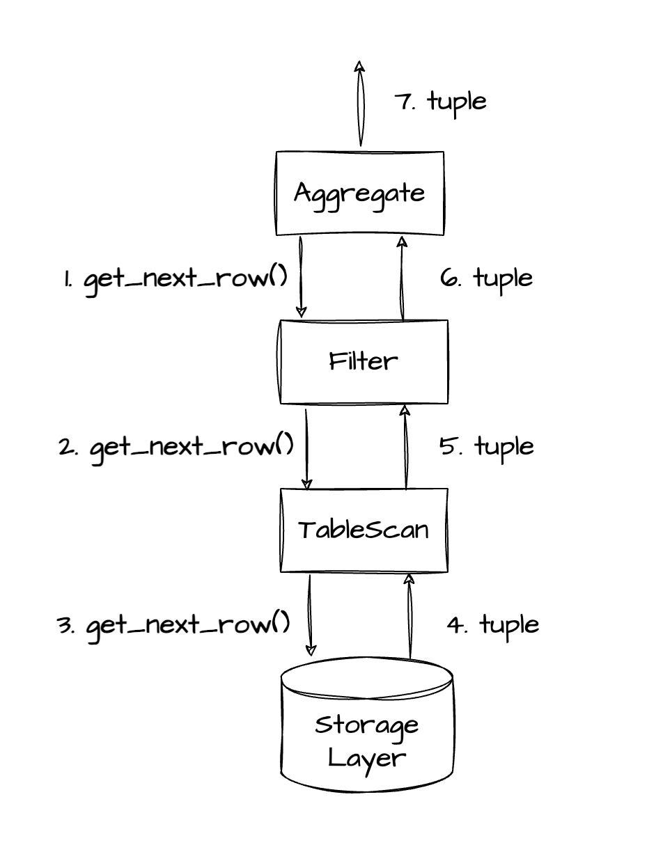
Note:
Each tuple in the preceding figure is a result row returned by a lower-level operator to a higher-level operator.
The process in the preceding figure is described as follows:
- Steps 1‒3: The AGGREGATE operator first calls the get_next_row() method so that lower-level operators can call the get_next_row() method of their child operators level by level.
- Steps 4‒6: After obtaining data from the storage layer, the TABLE SCAN operator returns the result row to the FILTER operator. After calculating data based on the filter condition
c1 = 1000, the FILTER operator returns the result row to the AGGREGATE operator. - Step 7: The AGGREGATE operator repeatedly calls the next() method to retrieve the required data, completes the aggregation, and returns the result.
If you disable vectorization in OceanBase Database, you can find execution plan trees similar to the one in the preceding figure.
    -- Disable vectorization to force subsequent SQL queries to use the default single-row calculation mode, which is similar to that of the Volcano model.
    alter system set _rowsets_enabled = false;

    -- You can observe that no rowset value exists in the following plan.
    explain select count(*) from t1 where c1 = 1000;
    +------------------------------------------------------------------------------------+
    | Query Plan                                                                         |
    +------------------------------------------------------------------------------------+
    | =================================================                                  |
    | |ID|OPERATOR         |NAME|EST.ROWS|EST.TIME(us)|                                  |
    | -------------------------------------------------                                  |
    | |0 |SCALAR GROUP BY  |    |1       |6           |                                  |
    | |1 |└─TABLE FULL SCAN|t1  |1       |6           |                                  |
    | =================================================                                  |
    | Outputs & filters:                                                                 |
    | -------------------------------------                                              |
    |   0 - output([T_FUN_COUNT_SUM(T_FUN_COUNT(*))]), filter(nil)                       |
    |       group(nil), agg_func([T_FUN_COUNT_SUM(T_FUN_COUNT(*))])                      |
    |   1 - output([T_FUN_COUNT(*)]), filter([t1.c1 = 1000])                             |
    |       access([t1.c1]), partitions(p0)                                              |
    |       is_index_back=false, is_global_index=false, filter_before_indexback[false],  |
    |       range_key([t1.__pk_increment]), range(MIN ; MAX)always true                  |
    +------------------------------------------------------------------------------------+
    14 rows in set (0.010 sec)
The plan in OceanBase Database contains only two operators and is simpler than that in the preceding figure. As every operator in OceanBase Database contains the functionality of the FILTER operator, no separate FILTER operator is needed. As shown in the preceding plan, the TABLE SCAN operator contains filter([t1.c1 = 1000]). The SCALAR GROUP BY operator in the plan corresponds to the AGGREGATE operator in the figure. It performs aggregations in scenarios where GROUP BY is not used.
The Volcano model has clear processing logic, where operators are decoupled so that each operator focuses only on its own tasks. However, the model has two obvious drawbacks:
- The virtual function get_next_row() is called for each row processed by every operator, and excessive calls can waste CPU resources. This issue is especially apparent in online analytical processing (OLAP) queries with a large data volume.
- Processing data row by row does not fully unleash the potential of modern CPUs.
Vectorized Execution Engine and Its Benefits
Vectorized models were first introduced in the paper MonetDB/X100: Hyper-Pipelining Query Execution. Unlike the Volcano model which iterates data row by row, a vectorized model adopts batch iterations, allowing a batch of data to be passed between operators at a time. Due to their effective use of CPU resources and modern CPU features, vectorized models have been widely adopted in the design of modern database engines.
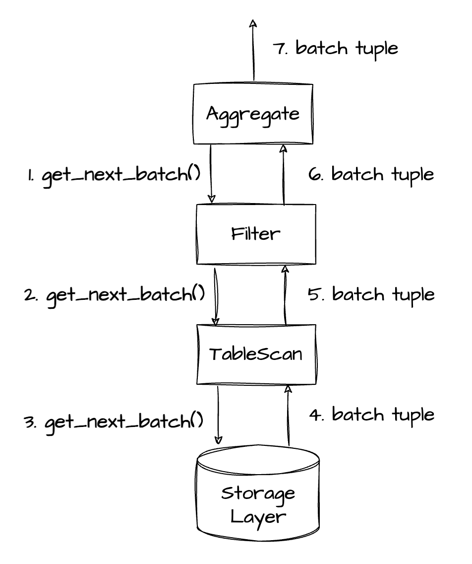
As shown in the preceding figure, the vectorized model pulls data from the root node of an operator tree level by level in a similar way as the traditional Volcano model. The difference is that the vectorized engine calls the get_next_batch() function to pass a batch of data at a time and keeps the batch as compact as possible in the memory, rather than calling the get_next_row() function to pass one row at a time.
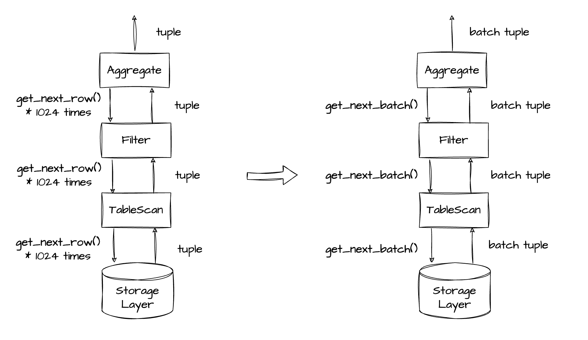
Reduce the Overhead of Virtual Function Calls
The vectorized engine drastically reduces the number of function calls. Assuming that you want to query a table with 100 million rows of data. In a database based on the Volcano model, each operator must call the get_next_row() function 100 million times to complete the query. If you use the vectorized engine and set the vector size to 1,024 rows, the number of calls to the get_next_batch() function for the same query, which is calculated by dividing 100 million by 1,024, is 97,657. This greatly decreases the number of virtual function calls and reduces CPU overhead.
In terms of the user question mentioned at the start of this article, the rowset in the plan indicates the number of rows in a batch or vector.
    -- Enable vectorization.
    alter system set _rowsets_enabled = true;

    -- Set the vector size to 16 rows.
    alter system set _rowsets_max_rows = 16;

    -- The rowset information (rowset = 16) in the plan indicates that the vector size is 16 rows.
    explain select count(*) from t1 where c1 = 1000;
    +------------------------------------------------------------------------------------+
    | Query Plan                                                                         |
    +------------------------------------------------------------------------------------+
    | =================================================                                  |
    | |ID|OPERATOR         |NAME|EST.ROWS|EST.TIME(us)|                                  |
    | -------------------------------------------------                                  |
    | |0 |SCALAR GROUP BY  |    |1       |4           |                                  |
    | |1 |└─TABLE FULL SCAN|t1  |1       |4           |                                  |
    | =================================================                                  |
    | Outputs & filters:                                                                 |
    | -------------------------------------                                              |
    |   0 - output([T_FUN_COUNT_SUM(T_FUN_COUNT(*))]), filter(nil), rowset=16            |
    |       group(nil), agg_func([T_FUN_COUNT_SUM(T_FUN_COUNT(*))])                      |
    |   1 - output([T_FUN_COUNT(*)]), filter([t1.c1 = 1000]), rowset=16                  |
    |       access([t1.c1]), partitions(p0)                                              |
    |       is_index_back=false, is_global_index=false, filter_before_indexback[false],  |
    |       range_key([t1.__pk_increment]), range(MIN ; MAX)always true                  |
    +------------------------------------------------------------------------------------+
    14 rows in set (0.021 sec)
Unleash the Potential of Modern CPUs
Compact data layout for better cache efficiency
During vectorized execution, OceanBase Database compactly stores batch data in memory, with intermediate data organized in columns. For example, if a batch contains 256 rows, the 256 rows of data of the c1 column are stored contiguously in memory, followed by those of the c2 column, which are also stored contiguously. For the concat(c1, c2) expression, calculation is performed on the 256 rows at a time, with the result stored in the memory space pre-allocated to the expression.
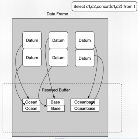
Since the intermediate data is contiguous, the CPU can quickly load the data into the L2 cache through the prefetch instruction to reduce memory stalls and improve CPU utilization. Inside an operator function, data is processed in batches rather than row by row, enhancing the efficiency of data cache (DCache) and instruction cache (ICache) in the CPU while reducing cache misses.
Reduced impact of branch mispredictions on the CPU pipeline
The paper DBMSs On A Modern Processor: Where Does Time Go? discusses the impact of branch mispredictions on database performance. Branch mispredictions have a serious impact on the database performance because the CPU halts the execution of an instruction stream and refreshes the pipeline upon a misprediction. The paper Micro Adaptivity in Vectorwise released on the 2013 ACM SIGMOD Conference on Management of Data (SIGMOD'13) also elaborates on the execution efficiency of branching at different levels of selectivity. A figure is provided below for your information.

The logic of the SQL engine of a database is complicated. Therefore, conditionals appear frequently in the Volcano model.
    // The following pseudocode outlines the single-row calculation process, where the IF statement is executed 256 times to process 256 rows of data:
    for (auto row_no : 256) {
      get_next_row() {
        if (A) {
          eval_func_A();
        } else if (B) {
          eval_func_B();
        }
      }
    }
In vectorized execution, conditionals are minimized within operators and expressions. For example, no IF statement is within any FOR loops, thus protecting the CPU pipeline from branch mispredictions and greatly improving CPU capabilities.
    // The following pseudocode outlines the vectorized calculation process, where the IF statement is executed only once to process 256 rows of data:
    get_next_batch() {
      if (A) {
        for (auto row_no : 256) {
          eval_func_A();
        }
      } else if (B) {
          for (auto row_no : 256) {
          eval_func_B();
        }
      }
    }
Accelerated computation through SIMD instructions
The vectorized engine handles contiguous data in the memory, and hence can easily load a batch of data into a vector register. It then sends a single instruction, multiple data (SIMD) instruction to perform vector computation instead of using the traditional scalar algorithm. The SIMD instruction enables the CPU to perform the same computation on the batch of data in parallel, reducing the number of CPU cycles required for processing the data.
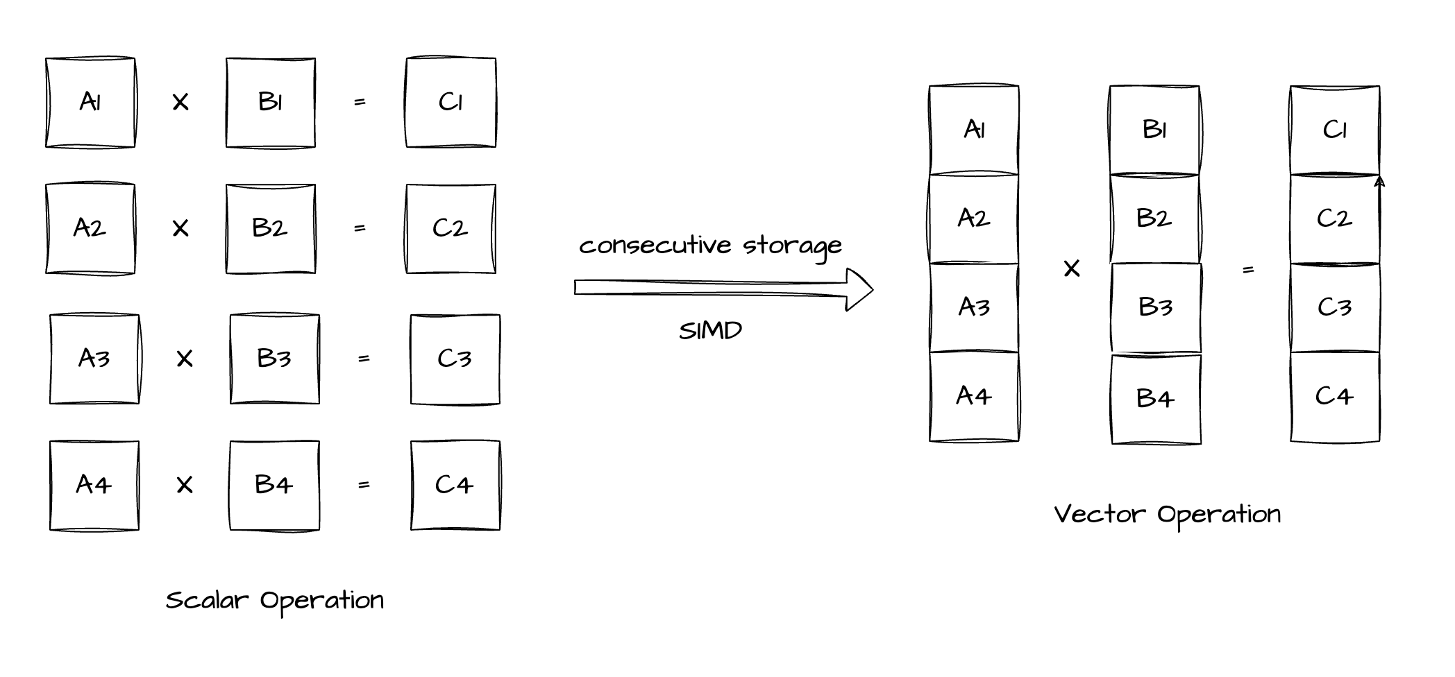
The right side of the preceding figure shows a typical SIMD computation, where two sets of four contiguous data elements are processed in parallel. The CPU simultaneously performs the same operation on each pair of data elements (A1 and B1, A2 and B2, A3 and B3, and A4 and B4) based on the SIMD instruction. The results of the four parallel operations are also stored contiguously.
If a processor supports 4-element SIMD multiplication, it has vector registers that can simultaneously store four integers. As OceanBase Database stores data contiguously during vectorized execution, SIMD code can be written as follows:
- Load data (_mm_loadu_si128): First, load the vector with the A1, A2, A3, and A4 elements and the vector with the B1, B2, B3, and B4 elements into two SIMD registers.
- Perform SIMD multiplication (_mm_mullo_epi32): Next, use the SIMD multiplication instruction to simultaneously multiply all elements in both registers.
- Store data (_mm_storeu_si128): Last, store the results from the SIMD registers in the allocated memory to form the result vector.
    // The sample C++ pseudocode based on Streaming SIMD Extensions (SSE) for x86 performs element-wise multiplication of integer vectors by using the SIMD technology.
    #include <immintrin.h> // Include the SSE header file.

    // Use the function to perform element-wise multiplication of two integer vectors.
    void simdIntVectorMultiply(const int* vec1, const int* vec2, int* result, size_t length) {
      // As SSE registers process four 32-bit integers at a time, make sure that the vector length is a multiple of four.
      assert(length % 4 == 0);

      // Execute the loop that uses SSE instructions for optimization.
        for (size_t i = 0; i < length; i += 4) {

        // Load four integers into the 128-bit XMM register.
        __m128i vec1_simd = _mm_loadu_si128(reinterpret_cast<const __m128i*>(vec1 + i));
        __m128i vec2_simd = _mm_loadu_si128(reinterpret_cast<const __m128i*>(vec2 + i));

        // Perform vector multiplication.
        __m128i product_simd = _mm_mullo_epi32(vec1_simd, vec2_simd);

        // Store the results in the memory.
        _mm_storeu_si128(reinterpret_cast<__m128i*>(result + i), product_simd);
      }
    }
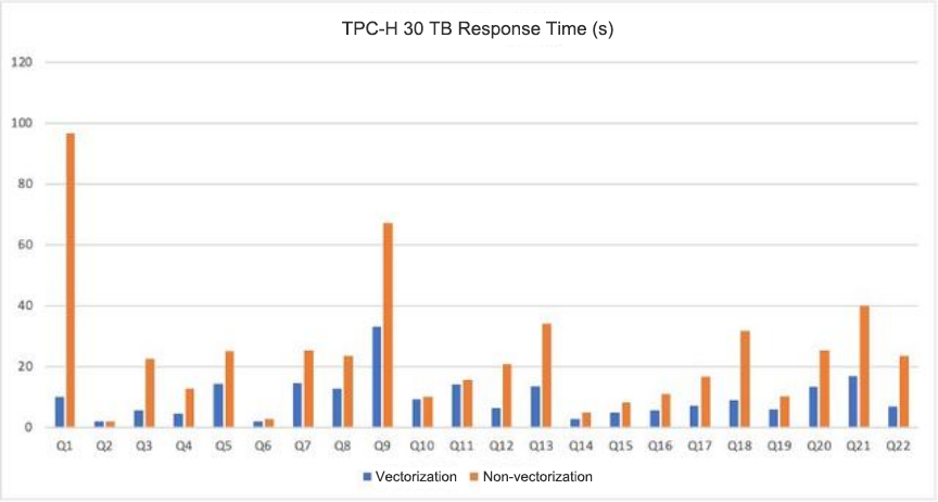
TPC-H Performance Test
In the TPC-H test based on the TPC-H 30 TB dataset on OceanBase Database, vectorized execution outperforms single-row execution by 2.48 times. For compute-intensive Q1 queries, performance is improved by over 10 times.
In OceanBase Database V4.3, the OceanBase team has optimized and restructured the vectorized execution engine, which has been supported since OceanBase Database V3.x.
Summary
This article was inspired by the question about the meaning of rowset=16 in a plan, which was raised during the seventh live streaming of OceanBase DBA: From Basics to Practices. After answering the question, this article also briefly introduces the vectorized execution technology of OceanBase Database.
I hope both database administrators (DBAs) and kernel developers find this helpful. For any questions, feel free to leave a comment.