OceanBase Distributed Pushdown Technology
I have been studying the book "An Interpretation of OceanBase Database Source Code" and noticed that it contains very little content about the SQL executor. Therefore, I want to write some blog posts about the SQL executor as a supplement to this book. In my last post Adaptive Techniques in the OceanBase Database Execution Engine, I introduced some representative adaptive techniques in the executor, based on the assumption that you have a basic understanding of the two-phase pushdown technique for HASH GROUP BY. If you are unfamiliar with the multi-phase pushdown technique of the executor, you are welcome to read this post to learn about common adaptive distributed pushdown techniques in OceanBase Database.
What is distributed pushdown?
To better utilize parallel execution capabilities and reduce CPU and network overheads during distributed execution, the optimizer often pushes down some operators to lower-layer compute nodes when it generates execution plans. This is to make full use of the computing resources of the cluster to improve the execution efficiency. Next, I'm going to introduce the most common distributed pushdown techniques in OceanBase Database.
LIMIT pushdown
Let me first talk about the pushdown of the LIMIT operator. The following are two SQL statements for creating a table named order and reading 100 rows from the orders table, respectively.
CREATE TABLE `orders` (
    `o_orderkey` bigint(20) NOT NULL,
    `o_custkey` bigint(20) NOT NULL,
    `o_orderdate` date NOT NULL,
    PRIMARY KEY (`o_orderkey`, `o_orderdate`, `o_custkey`),
    KEY `o_orderkey` (`o_orderkey`) LOCAL  BLOCK_SIZE 16384
)  partition by range columns(o_orderdate)
    subpartition by hash(o_custkey) subpartitions 64
(partition ord1 values less than ('1992-01-01'),
partition ord2 values less than ('1992-02-01'),
partition ord3 values less than ('1992-03-01'),
partition ord77 values less than ('1998-05-01'),
partition ord78 values less than ('1998-06-01'),
partition ord79 values less than ('1998-07-01'),
partition ord80 values less than ('1998-08-01'),
partition ord81 values less than (MAXVALUE));

select * from orders limit 100;
The following plan shows a very common scenario of distributed pushdown.
explain select * from orders limit 100;
+-----------------------------------------------------------------------------------------------------------------------------------------------------------------+
| Query Plan                                                                                                                                                      |
+-----------------------------------------------------------------------------------------------------------------------------------------------------------------+
| =================================================================                                                                                               |
| |ID|OPERATOR                     |NAME    |EST.ROWS|EST.TIME(us)|                                                                                               |
| -----------------------------------------------------------------                                                                                               |
| |0 |LIMIT                        |        |1       |2794        |                                                                                               |
| |1 |└─PX COORDINATOR             |        |1       |2794        |                                                                                               |
| |2 |  └─EXCHANGE OUT DISTR       |:EX10000|1       |2793        |                                                                                               |
| |3 |    └─LIMIT                  |        |1       |2792        |                                                                                               |
| |4 |      └─PX PARTITION ITERATOR|        |1       |2792        |                                                                                               |
| |5 |        └─TABLE FULL SCAN    |orders  |1       |2792        |                                                                                               |
| =================================================================                                                                                               |
| Outputs & filters:                                                                                                                                              |
| -------------------------------------                                                                                                                           |
|   0 - output([orders.o_orderkey], [orders.o_custkey], [orders.o_orderdate]), filter(nil)                                                                        |
|       limit(100), offset(nil)                                                                                                                                   |
|   1 - output([orders.o_orderkey], [orders.o_custkey], [orders.o_orderdate]), filter(nil)                                                                        |
|   2 - output([orders.o_orderkey], [orders.o_custkey], [orders.o_orderdate]), filter(nil)                                                                        |
|       dop=1                                                                                                                                                     |
|   3 - output([orders.o_orderkey], [orders.o_custkey], [orders.o_orderdate]), filter(nil)                                                                        |
|       limit(100), offset(nil)                                                                                                                                   |
|   4 - output([orders.o_orderkey], [orders.o_orderdate], [orders.o_custkey]), filter(nil)                                                                        |
|       force partition granule                                                                                                                                   |
|   5 - output([orders.o_orderkey], [orders.o_orderdate], [orders.o_custkey]), filter(nil)                                                                        |
|       access([orders.o_orderkey], [orders.o_orderdate], [orders.o_custkey]), partitions(p0sp[0-63], p1sp[0-63], p2sp[0-63], p3sp[0-63], p4sp[0-63], p5sp[0-63], |
|        p6sp[0-63], p7sp[0-63])                                                                                                                                  |
|       limit(100), offset(nil), is_index_back=false, is_global_index=false,                                                                                      |
|       range_key([orders.o_orderkey], [orders.o_orderdate], [orders.o_custkey]), range(MIN,MIN,MIN ; MAX,MAX,MAX)always true                                     |
+-----------------------------------------------------------------------------------------------------------------------------------------------------------------+
You can see that Operators 0 and 3 in the plan are both LIMIT. Operator 0 is pushed down to generate Operator 3 to reduce the number of rows scanned by Operator 5, a TABLE SCAN operator, from each partition of the orders table. Each thread of the TABLE SCAN operator scans at most 100 rows. This reduces the overhead in data scan by the TABLE SCAN operator and the network overhead in sending data to Operator 1 for aggregation. At present in OceanBase Database, the EXCHANGE operator will send a packet after it receives 64 KB data from a lower-layer operator. If the LIMIT operator is not pushed down, massive data may be scanned, leading to a high network overhead.
In actual business scenarios, a LIMIT operator is usually used in combination with the ORDER BY keyword. If the ORDER BY keyword is used in the preceding example, a TOP-N SORT operator with much higher performance than a SORT operator will be generated in the plan.
explain select * from orders order by o_orderdate limit 100;
+-----------------------------------------------------------------------------------------------------------------------------------------------------------------+
| Query Plan                                                                                                                                                      |
+-----------------------------------------------------------------------------------------------------------------------------------------------------------------+
| =================================================================                                                                                               |
| |ID|OPERATOR                     |NAME    |EST.ROWS|EST.TIME(us)|                                                                                               |
| -----------------------------------------------------------------                                                                                               |
| |0 |LIMIT                        |        |1       |2794        |                                                                                               |
| |1 |└─PX COORDINATOR MERGE SORT  |        |1       |2794        |                                                                                               |
| |2 |  └─EXCHANGE OUT DISTR       |:EX10000|1       |2793        |                                                                                               |
| |3 |    └─TOP-N SORT             |        |1       |2792        |                                                                                               |
| |4 |      └─PX PARTITION ITERATOR|        |1       |2792        |                                                                                               |
| |5 |        └─TABLE FULL SCAN    |orders  |1       |2792        |                                                                                               |
| =================================================================                                                                                               |
| Outputs & filters:                                                                                                                                              |
| -------------------------------------                                                                                                                           |
|   0 - output([orders.o_orderkey], [orders.o_custkey], [orders.o_orderdate]), filter(nil)                                                                        |
|       limit(100), offset(nil)                                                                                                                                   |
|   1 - output([orders.o_orderkey], [orders.o_custkey], [orders.o_orderdate]), filter(nil)                                                                        |
|       sort_keys([orders.o_orderdate, ASC])                                                                                                                      |
|   2 - output([orders.o_orderkey], [orders.o_custkey], [orders.o_orderdate]), filter(nil)                                                                        |
|       dop=1                                                                                                                                                     |
|   3 - output([orders.o_orderkey], [orders.o_custkey], [orders.o_orderdate]), filter(nil)                                                                        |
|       sort_keys([orders.o_orderdate, ASC]), topn(100)                                                                                                           |
|   4 - output([orders.o_orderkey], [orders.o_orderdate], [orders.o_custkey]), filter(nil)                                                                        |
|       force partition granule                                                                                                                                   |
|   5 - output([orders.o_orderkey], [orders.o_orderdate], [orders.o_custkey]), filter(nil)                                                                        |
|       access([orders.o_orderkey], [orders.o_orderdate], [orders.o_custkey]), partitions(p0sp[0-63], p1sp[0-63], p2sp[0-63], p3sp[0-63], p4sp[0-63], p5sp[0-63], |
|        p6sp[0-63], p7sp[0-63])                                                                                                                                  |
|       is_index_back=false, is_global_index=false,                                                                                                               |
|       range_key([orders.o_orderkey], [orders.o_orderdate], [orders.o_custkey]), range(MIN,MIN,MIN ; MAX,MAX,MAX)always true                                     |
+-----------------------------------------------------------------------------------------------------------------------------------------------------------------+
If the LIMIT operator is not pushed down, Operator 3 will be a SORT operator. In this case, each thread needs to sort and send all the scanned data to the upper-layer data flow object (DFO). A DFO is a sub-plan. Adjacent DFOs are separated with an EXCHANGE operator. For more information, see https://www.oceanbase.com/docs/common-oceanbase-database-1000000000034037.
The purpose of pushing down the LIMIT operator is to end execution in advance to reduce calculation and network overheads.
AGGREGATION pushdown
Let me take the following statement that contains GROUP BY as an example to describe distributed pushdown in aggregation.
select count(o_totalprice), sum(o_totalprice) from orders group by o_orderdate;
This SQL statement queries the daily order count and sales amount. If you want to execute the statement in parallel, the most straightforward approach would be to distribute data in the table based on the hash values of the GROUP BY column (o_orderdate). This way, all rows with the same o_orderdate value are sent to the same thread. The threads can aggregate received data in parallel.
However, this plan requires to perform a shuffle on all data in the table, which may lead to a very high network overhead. Moreover, if data skew occurs in the table, for example, a large number of orders were placed on a specific day, the workload of the thread responsible for processing orders of this day will be much higher than that of other threads. This long-tail task may directly lead to a long execution time for the query.
To address these issues, the GROUP BY operator is pushed down to generate the following plan:
explain select count(o_totalprice), sum(o_totalprice) from orders group by o_orderdate;
+-----------------------------------------------------------------------------------------------------------------------------------------------------------+
| Query Plan                                                                                                                                                |
+-----------------------------------------------------------------------------------------------------------------------------------------------------------+
| =====================================================================                                                                                     |
| |ID|OPERATOR                         |NAME    |EST.ROWS|EST.TIME(us)|                                                                                     |
| ---------------------------------------------------------------------                                                                                     |
| |0 |PX COORDINATOR                   |        |1       |2796        |                                                                                     |
| |1 |└─EXCHANGE OUT DISTR             |:EX10001|1       |2795        |                                                                                     |
| |2 |  └─HASH GROUP BY                |        |1       |2795        |                                                                                     |
| |3 |    └─EXCHANGE IN DISTR          |        |1       |2794        |                                                                                     |
| |4 |      └─EXCHANGE OUT DISTR (HASH)|:EX10000|1       |2794        |                                                                                     |
| |5 |        └─HASH GROUP BY          |        |1       |2793        |                                                                                     |
| |6 |          └─PX PARTITION ITERATOR|        |1       |2792        |                                                                                     |
| |7 |            └─TABLE FULL SCAN    |orders  |1       |2792        |                                                                                     |
| =====================================================================                                                                                     |
| Outputs & filters:                                                                                                                                        |
| -------------------------------------                                                                                                                     |
|   0 - output([INTERNAL_FUNCTION(T_FUN_COUNT_SUM(T_FUN_COUNT(orders.o_totalprice)), T_FUN_SUM(T_FUN_SUM(orders.o_totalprice)))]), filter(nil)              |
|   1 - output([INTERNAL_FUNCTION(T_FUN_COUNT_SUM(T_FUN_COUNT(orders.o_totalprice)), T_FUN_SUM(T_FUN_SUM(orders.o_totalprice)))]), filter(nil)              |
|       dop=1                                                                                                                                               |
|   2 - output([T_FUN_COUNT_SUM(T_FUN_COUNT(orders.o_totalprice))], [T_FUN_SUM(T_FUN_SUM(orders.o_totalprice))]), filter(nil)                               |
|       group([orders.o_orderdate]), agg_func([T_FUN_COUNT_SUM(T_FUN_COUNT(orders.o_totalprice))], [T_FUN_SUM(T_FUN_SUM(orders.o_totalprice))])             |
|   3 - output([orders.o_orderdate], [T_FUN_COUNT(orders.o_totalprice)], [T_FUN_SUM(orders.o_totalprice)]), filter(nil)                                     |
|   4 - output([orders.o_orderdate], [T_FUN_COUNT(orders.o_totalprice)], [T_FUN_SUM(orders.o_totalprice)]), filter(nil)                                     |
|       (#keys=1, [orders.o_orderdate]), dop=1                                                                                                              |
|   5 - output([orders.o_orderdate], [T_FUN_COUNT(orders.o_totalprice)], [T_FUN_SUM(orders.o_totalprice)]), filter(nil)                                     |
|       group([orders.o_orderdate]), agg_func([T_FUN_COUNT(orders.o_totalprice)], [T_FUN_SUM(orders.o_totalprice)])                                         |
|   6 - output([orders.o_orderdate], [orders.o_totalprice]), filter(nil)                                                                                    |
|       force partition granule                                                                                                                             |
|   7 - output([orders.o_orderdate], [orders.o_totalprice]), filter(nil)                                                                                    |
|       access([orders.o_orderdate], [orders.o_totalprice]), partitions(p0sp[0-63], p1sp[0-63], p2sp[0-63], p3sp[0-63], p4sp[0-63], p5sp[0-63], p6sp[0-63], |
|        p7sp[0-63])                                                                                                                                        |
|       is_index_back=false, is_global_index=false,                                                                                                         |
|       range_key([orders.o_orderkey], [orders.o_orderdate], [orders.o_custkey]), range(MIN,MIN,MIN ; MAX,MAX,MAX)always true                               |
+-----------------------------------------------------------------------------------------------------------------------------------------------------------+
In this plan, each thread will pre-aggregate the data it reads before distributing the data. The pre-aggregate job is done by Operator 5, a GROUP BY operator. Then, Operator 5 will send the aggregation results to its upper-layer operator. Operator 2, another GROUP BY operator, will aggregate the received data again. After Operator 5 pre-aggregates the data, the data amount will remarkably decrease. This can decrease the network overhead caused by data shuffle and reduce the impact of data skew on the execution time.
Then, let me demonstrate the execution process of the preceding SQL statement.
select count(o_totalprice), sum(o_totalprice) from orders group by o_orderdate;
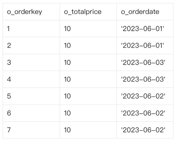
The original data comprises seven rows. The amount of each order is CNY 10. The orders were placed on June 1, June 2, and June 3.
The following figure shows the execution process, where the DOP is set to 2.
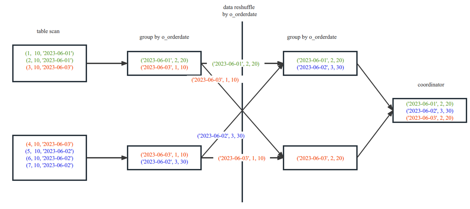
The first thread in the upper-left corner scans three rows, and the second thread in the lower-left corner scans four rows. Data with the same date, namely, data in the same group, is marked with the same color.
The first thread aggregates the three rows it scans, which are distributed in two groups. The dates of two rows are June 1. Therefore, for June 1, the order count is 2 and the sales amount is 20. The date of one row is June 3. Therefore, for June 3, the order count is 1 and the sales amount is 10. The four rows scanned by the second thread are also distributed in two groups. Two rows are generated after aggregation. The job of this part is completed by Operator 5 in the plan.
Then, the two threads distribute the data based on the hash values of the o_orderdate column. Data with the same date is sent to the same thread. The job of this part is completed by Operators 3 and 4 in the plan.
Each thread on the right side will aggregate the received data again. The two rows of June 3 scanned by the two threads on the left side, which are marked red, are sent to the thread in the lower-right corner. The two rows are aggregated again by the operator on the right side. After aggregation, the order count is 2 and the sales amount is 20. The two rows are finally aggregated into one row. The job of this part is completed by Operator 2 in the plan.
Then, all data is sent to the coordinator, which will summarize the data and send the final calculation results to the client.
JOIN FILTER pushdown
In a JOIN operator, the join filters of the left-side table will be pushed down to the right-side table to perform pre-filtering and partition pruning for data in the right-side table.
Pre-filtering
When a hash join is executed, the data in the left-side table is always read first to build a hash table. Then, the data in the right-side table is used to probe the hash table, and if successful, the data will be sent to the upper-layer operator. If a reshuffle is performed on the data in the right-side table of the hash join, the network overhead may be high, which is subject to the data amount of the right-side table. In this case, join filters can be used to reduce the network overhead caused by data shuffle.
Take the plan shown in the following figure as an example.

In the plan, Operator 2, a HASH JOIN operator, reads data from the left-side table. During the read, it will use the t1.c1 join key to create a join filter, which is done by Operator 3, a JOIN FILTER CREATE operator. The most common form of join filter is Bloom filter. After the join filter is created, it is sent to the right-side DFO, which contains Operator 6 and other lower-layer operators.
Operator 10, a TABLE SCAN operator, has a filter sys_op_bloom_filter(t2.c1), which specifies to use values of t2.c1 in the right-side table to quickly probe the hash table based on the Bloom filter. If a value of t2.c1 does not match any value of t1.c1, the row where the t2.c1 value is located in the t2 table can be pre-filtered and does not need to be sent to the HASH JOIN operator.
Partition pruning
Join filters can be used not only for row filtering but also for partition pruning (or filtering). Assume that t1 is a partitioned table and the join key is also its partitioning key. A plan shown in the following figure can be generated.
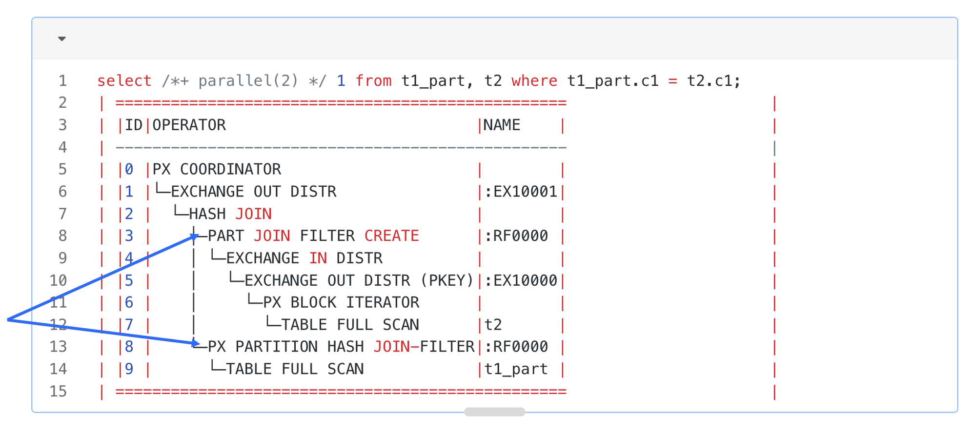
In this plan, Operator 3 is a PARTITION JOIN FILTER CREATE operator. It will detect the partitioning method of the right-side t1 table of the hash join. When it obtains a row in the left-side table from the lower-layer operator, it will use the c1 value to calculate the partition to which this row belongs in the right-side t1 table, and record the partition ID in the join filter. The join filter that contains the partition ID will be used on Operator 8 for partition pruning for the right-side table of the hash join. When the table scan operator scans each partition in the right-side table, it will verify whether the partition ID exists in the join filter. If no, it can skip the entire partition.
A join filter can be used for data pre-filtering and partition pruning, thereby reducing the overheads in data scan, network transmission, and hash table probe. At present, OceanBase Database supports only Bloom filters in versions earlier than V4.2. OceanBase Database supports two new types of join filters since V4.2: In filter and Range filter. The new join filters can help significantly improve the performance in some scenarios, especially when the left-side table contains a few distinct values or contains continuous values.
Other distributed pushdown techniques
Apart from the preceding common distributed pushdown techniques that are easy to understand, OceanBase Database also supports more adaptive distributed pushdown techniques, such as adaptive two-phase pushdown for window functions and three-phase pushdown for aggregate functions.
This post will not provide a detailed introduction to the more complex distributed pushdown techniques of OceanBase Database. Below are sample execution plans of the two distributed pushdown techniques mentioned earlier for those who are interested in conducting further research.
Adaptive two-phase pushdown for window functions:
select /*+parallel(3) */
        c1, sum(c2) over (partition by c1) from t1 order by c1;
Query Plan
===================================================
|ID|OPERATOR                             |NAME    |
---------------------------------------------------
|0 |PX COORDINATOR MERGE SORT            |        |
|1 | EXCHANGE OUT DISTR                  |:EX10001|
|2 |  MATERIAL                           |        |
|3 |   WINDOW FUNCTION CONSOLIDATOR      |        |
|4 |    EXCHANGE IN MERGE SORT DISTR     |        |
|5 |     EXCHANGE OUT DISTR (HASH HYBRID)|:EX10000|
|6 |      WINDOW FUNCTION                |        |
|7 |       SORT                          |        |
|8 |        PX BLOCK ITERATOR            |        |
|9 |         TABLE SCAN                  |t1      |
===================================================
Three-phase pushdown for aggregate functions:
select /*+ parallel(2) */
    c1, sum(distinct c2),count(distinct c3), sum(c4) from t group by c1;
Query Plan
===========================================================================
|ID|OPERATOR                               |NAME    |EST.ROWS|EST.TIME(us)|
---------------------------------------------------------------------------
|0 |PX COORDINATOR                         |        |1       |8           |
|1 |└─EXCHANGE OUT DISTR                   |:EX10002|1       |7           |
|2 |  └─HASH GROUP BY                      |        |1       |6           |
|3 |    └─EXCHANGE IN DISTR                |        |2       |6           |
|4 |      └─EXCHANGE OUT DISTR (HASH)      |:EX10001|2       |6           |
|5 |        └─HASH GROUP BY                |        |2       |4           |
|6 |          └─EXCHANGE IN DISTR          |        |2       |4           |
|7 |            └─EXCHANGE OUT DISTR (HASH)|:EX10000|2       |3           |
|8 |              └─HASH GROUP BY          |        |2       |2           |
|9 |                └─PX BLOCK ITERATOR    |        |1       |1           |
|10|                  └─TABLE FULL SCAN    |t       |1       |1           |
===========================================================================
Preview of the next post
This post introduces several typical distributed pushdown techniques in the executor of OceanBase Database, based on the assumption that you have a basic understanding of distributed execution of the database. If you are unfamiliar with parallel execution techniques of the executor, please look forward to the next post Parallel Execution Techniques of OceanBase Database.