7.6 Common SQL tuning methods

'7.5 Read and manage SQL execution plans in OceanBase Database' describes how to use the EXPLAIN statement to query the logical execution plan generated by the optimizer for an SQL statement and how to use hints and outlines to control the optimizer to generate a specified plan.

This topic further describes SQL performance tuning in OceanBase Database. The first part of this topic describes statistics and the plan cache mechanism. The second part describes the performance tuning methods supported in OceanBase Database.

Statistics

In a database, the optimizer tries to generate the optimal execution plan for each SQL query, most commonly, based on accurate statistics. Statistics here refer to optimizer statistics, which are a collection of data that describes the tables and columns in a database, and are key for the cost model to select the optimal execution plan.

The optimizer cost model optimizes plan selection based on the statistics on the tables, columns, predicates, and other objects involved in a query. Accurate and effective statistics can help the optimizer select the optimal execution plan.

Note

This section first describes the concepts of histograms and buckets.

• Histograms are a special form of column statistics. By default, the optimizer considers that data is evenly distributed in a column and estimates the number of rows based on this feature. However, in real scenarios, data distribution is uneven in most tables. As a result, the optimizer inaccurately estimates the number of rows and cannot select the optimal execution plan. A histogram helps the optimizer estimate the number of rows more accurately.

• In a histogram, data is stored in a series of ordered buckets to describe the statistical distribution features of the column. The optimizer can estimate a more accurate number of rows based on a histogram. A histogram contains 254 buckets by default. More buckets indicate higher accuracy of the statistics but also higher costs of statistics collection.

This section describes how to collect and query statistics but not how to manage statistics or how the optimizer uses statistics to estimate the number of rows.

In OceanBase Database V4.x, statistics can be collected both manually and automatically.

Manually collect statistics

You can manually collect statistics to help the optimizer generate a better plan.

The optimizer allows you to manually collect statistics by using the DBMS_STATS package or executing the ANALYZE statement in a CLI tool. We recommend that you use the DBMS_STATS package because it provides more features. For more information about the DBMS_STATS package, see DBMS_STATS.

DBMS_STATS package (recommended)

The DBMS_STATS package provides two common stored procedures:

• GATHER_TABLE_STATS: collects statistics on a specified table. For information about the syntax and parameters of this procedure, see GATHER_TABLE_STATS.

• GATHER_SCHEMA_STATS: collects statistics on all tables in a database. For information about the syntax and parameters of this procedure, see GATHER_SCHEMA_STATS.

Here are some examples:

• Collect global statistics on the T1 table in the TEST database, with the number of buckets being 128 for all columns.

  call dbms_stats.gather_table_stats('TEST', 'T1', granularity=>'GLOBAL', method_opt=>'FOR ALL COLUMNS SIZE 128');

• Collect partition-level statistics on the T_PART1 table in the TEST database, with a degree of parallelism (DOP) of 64 and only histograms of columns with uneven data distribution collected.

  call dbms_stats.gather_table_stats('TEST', 'T_PART1', degree=>64, granularity=>'PARTITION', method_opt=>'FOR ALL COLUMNS SIZE SKEWONLY');

• Collect all statistics on the T_SUBPART1 table in the TEST database, with only 50% of data collected.

  call dbms_stats.gather_table_stats('TEST', 'T_SUBPART1', estimate_percent=> '50', granularity=>'ALL');

• Collect all statistics on all tables in the TEST database, with a DOP of 128.

  call dbms_stats.gather_schema_stats('TEST', degree=>128);

Notice

The first parameter in the syntax of both the GATHER_TABLE_STATS and GATHER_SCHEMA_STATS procedures is database_name instead of user_name. The information in the documentation for some OceanBase Database versions may be incorrect.

The DMBS_STATS package also provides the GATHER_INDEX_STATS procedure to collect index statistics and the GATHER_DATABASE_STATS_JOB_PROC procedure to collect statistics on all tables of all databases in a tenant.

ANALYZE statement

You can also execute the ANALYZE statement to collect statistics in OceanBase Database. For information about the syntax and parameters of this statement, see ANALYZE.

Before you execute this statement in MySQL mode, you must set the enable_sql_extension parameter to TRUE. This is because MySQL does not natively support this statement, and you can execute it only after you enable SQL extension.

ALTER SYSTEM SET enable_sql_extension = TRUE;

Here are some examples:

• Collect statistics on the T1 table, with the number of buckets being 128 for all columns.

  ANALYZE TABLE T1 COMPUTE STATISTICS FOR ALL COLUMNS SIZE 128;

• Collect global statistics on the T_PART1 table, with only histograms of columns with uneven data distribution collected.

  ANALYZE TABLE T_PART1 PARTITION('T_PART1') COMPUTE STATISTICS FOR ALL COLUMNS SIZE skewonly;

• Collect statistics on the p0sp0 and p1ps2 partitions of the T_SUBPART1 table.

  ANALYZE TABLE T_SUBPART1 SUBPARTITION('p0sp0','p1ps2') COMPUTE STATISTICS FOR ALL COLUMNS SIZE auto;

• Collect statistics on the c1 and c2 columns of the T1 table, with the number of buckets being 30 for the columns. The syntax of the ANALYZE statement is compatible with that in native MySQL.

  ANALYZE TABLE T1 UPDATE HISTOGRAM ON c1, c2 with 30 buckets;

Automatically collect statistics

The optimizer performs automatic daily statistics collection based on the maintenance window to keep statistics automatically updated. Like in a native Oracle database, the optimizer of OceanBase Database schedules an automatic statistics collection task each day. By default, the tasks from Monday to Friday start at 22:00, with a maximum collection duration of 4 hours, and the tasks on Saturday and Sunday start at 6:00, with a maximum collection duration of 20 hours.

OceanBase Database provides the OCEANBASE.DBA_SCHEDULER_WINDOWS and OCEANBASE.DBA_SCHEDULER_JOBS views for you to query the status of automatic statistics collection tasks. Here are some examples:

• Query all maintenance windows.

  select WINDOW_NAME, LAST_START_DATE, NEXT_RUN_DATE
    from OCEANBASE.DBA_SCHEDULER_WINDOWS
    where LAST_START_DATE is not null order by LAST_START_DATE;

  For more information about the fields in the OCEANBASE.DBA_SCHEDULER_WINDOWS view, see oceanbase.DBA_SCHEDULER_WINDOWS. The output is as follows:

  +------------------+----------------------------+----------------------------+
  | WINDOW_NAME      | LAST_START_DATE            | NEXT_RUN_DATE              |
  +------------------+----------------------------+----------------------------+
  | TUESDAY_WINDOW   | 2024-03-12 22:00:00.084516 | 2024-03-19 22:00:00.000000 |
  | WEDNESDAY_WINDOW | 2024-03-13 22:00:00.090113 | 2024-03-20 22:00:00.000000 |
  | THURSDAY_WINDOW  | 2024-03-14 22:00:00.105114 | 2024-03-21 22:00:00.000000 |
  | FRIDAY_WINDOW    | 2024-03-15 22:00:00.080400 | 2024-03-22 22:00:00.000000 |
  | SATURDAY_WINDOW  | 2024-03-16 06:00:00.104678 | 2024-03-23 06:00:00.000000 |
  | SUNDAY_WINDOW    | 2024-03-17 06:00:00.089326 | 2024-03-24 06:00:00.000000 |
  | MONDAY_WINDOW    | 2024-03-18 22:00:00.083798 | 2024-03-25 22:00:00.000000 |
  +------------------+----------------------------+----------------------------+
  7 rows in set

• Query all scheduler jobs.

  select JOB_NAME, REPEAT_INTERVAL, LAST_START_DATE, NEXT_RUN_DATE, MAX_RUN_DURATION
    from OCEANBASE.DBA_SCHEDULER_JOBS
    where LAST_START_DATE is not null order by LAST_START_DATE;

  For more information about the fields in the OCEANBASE.DBA_SCHEDULER_JOBS view, see oceanbase.DBA_SCHEDULER_JOBS. The output is as follows:

  +---------------------------+-------------------------+----------------------------+----------------------------+------------------+
  | JOB_NAME                  | REPEAT_INTERVAL         | LAST_START_DATE            | NEXT_RUN_DATE              | MAX_RUN_DURATION |
  +---------------------------+-------------------------+----------------------------+----------------------------+------------------+
  | TUESDAY_WINDOW            | FREQ=WEEKLY; INTERVAL=1 | 2024-03-12 22:00:00.084516 | 2024-03-19 22:00:00.000000 |            14400 |
  | WEDNESDAY_WINDOW          | FREQ=WEEKLY; INTERVAL=1 | 2024-03-13 22:00:00.090113 | 2024-03-20 22:00:00.000000 |            14400 |
  | THURSDAY_WINDOW           | FREQ=WEEKLY; INTERVAL=1 | 2024-03-14 22:00:00.105114 | 2024-03-21 22:00:00.000000 |            14400 |
  | FRIDAY_WINDOW             | FREQ=WEEKLY; INTERVAL=1 | 2024-03-15 22:00:00.080400 | 2024-03-22 22:00:00.000000 |            14400 |
  | SATURDAY_WINDOW           | FREQ=WEEKLY; INTERVAL=1 | 2024-03-16 06:00:00.104678 | 2024-03-23 06:00:00.000000 |            72000 |
  | SUNDAY_WINDOW             | FREQ=WEEKLY; INTERVAL=1 | 2024-03-17 06:00:00.089326 | 2024-03-24 06:00:00.000000 |            72000 |
  | MONDAY_WINDOW             | FREQ=WEEKLY; INTERVAL=1 | 2024-03-18 22:00:00.083798 | 2024-03-25 22:00:00.000000 |            14400 |
  | OPT_STATS_HISTORY_MANAGER | FREQ=DAYLY; INTERVAL=1  | 2024-03-19 11:10:46.014510 | 2024-03-20 11:10:46.000000 |             NULL |
  +---------------------------+-------------------------+----------------------------+----------------------------+------------------+
  8 rows in set

The optimizer allows you to set the start time and collection duration of automatic statistics collection jobs to cope with your business requirements.

• Disable or enable automatic statistics collection.

  DBMS_SCHEDULER.DISABLE($window_name)

  DBMS_SCHEDULER.ENABLE($window_name);

• Set the start time of the next automatic statistics job.

  DBMS_SCHEDULER.SET_ATTRIBUTE($window_name, 'NEXT_DATE', $next_time);

• Set the duration of automatic statistics collection jobs.

  DBMS_SCHEDULER.SET_ATTRIBUTE($window_name, 'DURATION', $duation_time);

Here are some examples:

• Disable automatic statistics collection on Mondays.

  call dbms_scheduler.disable('MONDAY_WINDOW');

• Enable automatic statistics collection on Mondays.

  call dbms_scheduler.enable('MONDAY_WINDOW');

• Set the start time of the automatic statistics collection job on Mondays to 20:00.

  call dbms_scheduler.set_attribute('MONDAY_WINDOW', 'NEXT_DATE', '2022-09-12 20:00:00');

• Set the duration of the automatic statistics collection job on Mondays to 6 hours.

  call dbms_scheduler.set_attribute('MONDAY_WINDOW', 'DURATION', INTERVAL '6' HOUR);

Working mechanism of automatic statistics collection

The optimizer determines whether the statistics on a table have expired based on the percentage of the changed table data since the last statistics collection. The default percentage is 10%. If the percentage of the changed table data exceeds 10%, the optimizer determines that the statistics on the table have expired and need to be re-collected. Note that this percentage of changed data is a partition-level parameter if the target table is a partitioned table. For example, if the percentage of added, deleted, and updated data of a partition exceeds 10% of the total data of the partition, the statistics on this partition are re-collected.

Note

The default percentage of changed data can be configured as needed by setting a preference. For more information, see Configure statistics collection strategies.

The optimizer also provides the OCEANBASE.DBA_TAB_MODIFICATIONS view for you to query the number of ADD, DELETE, and UPDATE operations on a table. For more information about the fields in the OCEANBASE.DBA_TAB_MODIFICATIONS view, see oceanbase.DBA_TAB_MODIFICATIONS. Here is an example:

select TABLE_OWNER as DB_NAME, TABLE_NAME, INSERTS, UPDATES, DELETES, TIMESTAMP
  from OCEANBASE.DBA_TAB_MODIFICATIONS
  where TABLE_OWNER = 'test' and TABLE_NAME = 't2';

The output is as follows:

+---------+------------+---------+---------+---------+------------+
| DB_NAME | TABLE_NAME | INSERTS | UPDATES | DELETES | TIMESTAMP  |
+---------+------------+---------+---------+---------+------------+
| test    | t2         |    1000 |       0 |       0 | 2024-03-15 |
+---------+------------+---------+---------+---------+------------+

Notice

The first column TABLE_OWNER of the OCEANBASE.DBA_TAB_MODIFICATIONS view indicates the database name rather than the user name. The information in the documentation for some OceanBase Database versions may be incorrect.

Query statistics

The optimizer provides a variety of views for you to query various types of statistics after statistics are collected.

View	Description
OCEANBASE.DBA_TAB_STATISTICS	Displays statistics of tables.
OCEANBASE.DBA_IND_STATISTICS	Displays statistics of indexes.
OCEANBASE.DBA_TAB_COL_STATISTICS	Displays global column statistics.
OCEANBASE.DBA_PART_COL_STATISTICS	Displays partition-level column statistics.
OCEANBASE.DBA_SUBPART_COL_STATISTICS	Displays subpartition-level column statistics.
OCEANBASE.DBA_TAB_HISTOGRAMS	Displays global column histogram statistics.
OCEANBASE.DBA_PART_HISTOGRAMS	Displays partition-level column histogram statistics.
OCEANBASE.DBA_SUBPART_HISTOGRAMS	Displays subpartition-level column histogram statistics.

Here is an example:

1. Create a partitioned table named t_part.

   create table t_part(c1 int) partition by hash(c1) partitions 4;

2. Insert 1,000 rows of data into the t_part table, with values of all the cells being 1.

   insert into t_part with recursive cte(n) as (select 1 from dual union all select n + 1 from cte where n < 1000) select 1 from cte;

3. Query statistics of the t_part table.

   select TABLE_NAME, PARTITION_NAME, PARTITION_POSITION, OBJECT_TYPE, NUM_ROWS, AVG_ROW_LEN, LAST_ANALYZED
     from OCEANBASE.DBA_TAB_STATISTICS
     where OWNER = 'test' and TABLE_NAME = 't_part';

   The query result is NULL because no statistics have been collected for the table. The output is as follows:

   +------------+----------------+--------------------+-------------+----------+-------------+---------------+
   | TABLE_NAME | PARTITION_NAME | PARTITION_POSITION | OBJECT_TYPE | NUM_ROWS | AVG_ROW_LEN | LAST_ANALYZED |
   +------------+----------------+--------------------+-------------+----------+-------------+---------------+
   | t_part     | p3             |                  4 | PARTITION   |     NULL |        NULL | NULL          |
   | t_part     | p2             |                  3 | PARTITION   |     NULL |        NULL | NULL          |
   | t_part     | p1             |                  2 | PARTITION   |     NULL |        NULL | NULL          |
   | t_part     | p0             |                  1 | PARTITION   |     NULL |        NULL | NULL          |
   | t_part     | NULL           |               NULL | TABLE       |     NULL |        NULL | NULL          |
   +------------+----------------+--------------------+-------------+----------+-------------+---------------+
   5 rows in set

4. Query the execution plan for the SQL statement.

   explain select * from t_part where c1 > 2;

5. Manually collect statistics.

   analyze table t_part COMPUTE STATISTICS for all columns size 128;

6. Query statistics of the t_part table again.

   select TABLE_NAME, PARTITION_NAME, PARTITION_POSITION, OBJECT_TYPE, NUM_ROWS, AVG_ROW_LEN, LAST_ANALYZED
     from OCEANBASE.DBA_TAB_STATISTICS
     where OWNER = 'test' and TABLE_NAME = 't_part';

   The output is as follows:

   +------------+----------------+--------------------+-------------+----------+-------------+----------------------------+
   | TABLE_NAME | PARTITION_NAME | PARTITION_POSITION | OBJECT_TYPE | NUM_ROWS | AVG_ROW_LEN | LAST_ANALYZED              |
   +------------+----------------+--------------------+-------------+----------+-------------+----------------------------+
   | t_part     | NULL           |               NULL | TABLE       |     1000 |          20 | 2024-03-22 14:11:03.188965 |
   | t_part     | p0             |                  1 | PARTITION   |        0 |           0 | 2024-03-22 14:11:03.188965 |
   | t_part     | p1             |                  2 | PARTITION   |     1000 |          20 | 2024-03-22 14:11:03.188965 |
   | t_part     | p2             |                  3 | PARTITION   |        0 |           0 | 2024-03-22 14:11:03.188965 |
   | t_part     | p3             |                  4 | PARTITION   |        0 |           0 | 2024-03-22 14:11:03.188965 |
   +------------+----------------+--------------------+-------------+----------+-------------+----------------------------+
   5 rows in set

7. Query the execution plan for the SQL statement.

   explain select * from t_part where c1 > 1;

   The c1 column of the table contains only cells with their values being 1. Therefore, the number of rows estimated based on the filter condition c1 > 1 in the plan is quite small, which is as expected. The output is as follows:

   +------------------------------------------------------------------------------------+
   | Query Plan                                                                         |
   +------------------------------------------------------------------------------------+
   | =============================================================                      |
   | |ID|OPERATOR                 |NAME    |EST.ROWS|EST.TIME(us)|                      |
   | -------------------------------------------------------------                      |
   | |0 |PX COORDINATOR           |        |1       |64          |                      |
   | |1 |└─EXCHANGE OUT DISTR     |:EX10000|1       |64          |                      |
   | |2 |  └─PX PARTITION ITERATOR|        |1       |64          |                      |
   | |3 |    └─TABLE FULL SCAN    |t_part  |1       |64          |                      |
   | =============================================================                      |
   | Outputs & filters:                                                                 |
   | -------------------------------------                                              |
   |   0 - output([INTERNAL_FUNCTION(t_part.c1)]), filter(nil), rowset=16               |
   |   1 - output([INTERNAL_FUNCTION(t_part.c1)]), filter(nil), rowset=16               |
   |       dop=1                                                                        |
   |   2 - output([t_part.c1]), filter(nil), rowset=16                                  |
   |       force partition granule                                                      |
   |   3 - output([t_part.c1]), filter([t_part.c1 > 1]), rowset=16                      |
   |       access([t_part.c1]), partitions(p[0-3])                                      |
   |       is_index_back=false, is_global_index=false, filter_before_indexback[false],  |
   |       range_key([t_part. __pk_increment]), range(MIN ; MAX)always true              |
   +------------------------------------------------------------------------------------+

8. Insert 1000 rows of data into the t_part table, with values of all cells being 99.

   insert into t_part with recursive cte(n)
     as (select 1 from dual union all select n + 1 from cte where n < 1000) select 99 from cte;

9. Query the execution plan again.

   explain select * from t_part where c1 > 1;

   The output is as follows:

   +------------------------------------------------------------------------------------+
   | Query Plan                                                                         |
   +------------------------------------------------------------------------------------+
   | =============================================================                      |
   | |ID|OPERATOR                 |NAME    |EST.ROWS|EST.TIME(us)|                      |
   | -------------------------------------------------------------                      |
   | |0 |PX COORDINATOR           |        |1       |64          |                      |
   | |1 |└─EXCHANGE OUT DISTR     |:EX10000|1       |64          |                      |
   | |2 |  └─PX PARTITION ITERATOR|        |1       |64          |                      |
   | |3 |    └─TABLE FULL SCAN    |t_part  |1       |64          |                      |
   | =============================================================                      |
   | Outputs & filters:                                                                 |
   | -------------------------------------                                              |
   |   0 - output([INTERNAL_FUNCTION(t_part.c1)]), filter(nil), rowset=16               |
   |   1 - output([INTERNAL_FUNCTION(t_part.c1)]), filter(nil), rowset=16               |
   |       dop=1                                                                        |
   |   2 - output([t_part.c1]), filter(nil), rowset=16                                  |
   |       force partition granule                                                      |
   |   3 - output([t_part.c1]), filter([t_part.c1 > 1]), rowset=16                      |
   |       access([t_part.c1]), partitions(p[0-3])                                      |
   |       is_index_back=false, is_global_index=false, filter_before_indexback[false],  |
   |       range_key([t_part. __pk_increment]), range(MIN ; MAX)always true              |
   +------------------------------------------------------------------------------------+

   Operator 3 is expected to output 1,000 rows based on the filter condition filter([t_part.c1 > 1]). However, the value in the EST.ROWS column is 1. This is because the optimizer has not collected statistics since the 1,000 rows of data with their cell values being 99 are inserted into the c1 column of the table and the number of rows estimated based on the condition c1 > 1 is still small, which is not as expected. In this case, you can manually collect statistics.

10. Manually collect statistics.

    analyze table t_part COMPUTE STATISTICS for all columns size 128;

11. Query the execution plan again.

    explain select * from t_part where c1 > 1;

    The estimated number of rows in the plan is as expected. The output is as follows:

    +------------------------------------------------------------------------------------+
    | Query Plan                                                                         |
    +------------------------------------------------------------------------------------+
    | =============================================================                      |
    | |ID|OPERATOR                 |NAME    |EST.ROWS|EST.TIME(us)|                      |
    | -------------------------------------------------------------                      |
    | |0 |PX COORDINATOR           |        |1000    |707         |                      |
    | |1 |└─EXCHANGE OUT DISTR     |:EX10000|1000    |515         |                      |
    | |2 |  └─PX PARTITION ITERATOR|        |1000    |87          |                      |
    | |3 |    └─TABLE FULL SCAN    |t_part  |1000    |87          |                      |
    | =============================================================                      |
    | Outputs & filters:                                                                 |
    | -------------------------------------                                              |
    |   0 - output([INTERNAL_FUNCTION(t_part.c1)]), filter(nil), rowset=256              |
    |   1 - output([INTERNAL_FUNCTION(t_part.c1)]), filter(nil), rowset=256              |
    |       dop=1                                                                        |
    |   2 - output([t_part.c1]), filter(nil), rowset=256                                 |
    |       force partition granule                                                      |
    |   3 - output([t_part.c1]), filter([t_part.c1 > 1]), rowset=256                     |
    |       access([t_part.c1]), partitions(p[0-3])                                      |
    |       is_index_back=false, is_global_index=false, filter_before_indexback[false],  |
    |       range_key([t_part. __pk_increment]), range(MIN ; MAX)always true              |
    +------------------------------------------------------------------------------------+

Plan cache

Overview

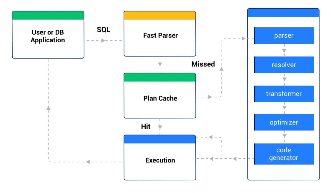
OceanBase Database provides a large number of rewrite rules and complex plan generation algorithms, implementing powerful optimization capabilities. However, more rewrite attempts and more complex plan generation algorithms inevitably make plan generation more time-consuming. In extreme transaction processing (TP) scenarios, plan generation for a primary key-based single point SQL query may take 1 ms, while the execution of the plan takes only 0.5 ms. In this scenario, if a plan needs to be regenerated each time the SQL statement is executed, a considerable amount of time will be consumed on plan generation for the statement. Therefore, OceanBase Database introduces the plan cache mechanism for similar SQL statements to share an execution plan.

After receiving an SQL request, OceanBase Database uses the fast parser module to quickly parameterize the SQL text. Fast parameterization replaces some constants in SQL text with the wildcard ?. For example, SELECT *FROM t1 WHERE c1 = 1 will be rewritten into SELECT* FROM t1 WHERE c1 = ? . Then, the optimizer checks the plan cache for a generated plan for this parameterized SQL statement. If a generated plan is found, the optimizer executes the plan directly. If no available plan is found, the optimizer generates an execution plan for the SQL statement and saves the plan to the plan cache for reuse by subsequent SQL statements.

In most cases, obtaining an execution plan directly from the plan cache takes at least an order of magnitude less time than regenerating an execution plan, and thus makes the SQL response quicker.

Bad case of the plan cache

As mentioned above, an execution plan is generated for a parameterized SQL statement and then saved to the plan cache for reuse by subsequent SQL statements. Although this method can save the plan generation time, it implies a bad case in data skew scenarios. Here is an example:

1. Create a table named t1.

   create table t1 (c1 int, c2 int, key idx1(c1), key idx2(c2));

2. Insert 1,000 rows of data into the table. The c1 column has only two unique values: the value 0 that accounts for 0.1% of all data and the value 1 that accounts for 99.9% of all data. The c2 column has 10 unique values, from 1 to 10, each of which accounts for 10% of total data.

   insert into t1 values(0, 0);
   
   insert into t1 with recursive cte(n)
     as (select 1 from dual union all select n + 1 from cte where n < 999) select 1, mod(n, 10) + 1 from cte;

3. Manually collect statistics.

   analyze table t1 COMPUTE STATISTICS for all columns size 128;

4. Execute an SQL statement.

   select* from t1 where c1 = 0 and c2 = 0;
   
   The parameterized SQL statement is as follows: `select *from t1 where c1 = ? and c2 = ? `.
   

5. Query the execution plan for the SQL statement from the plan cache.

   SELECT SQL_ID, PLAN_ID, STATEMENT, OUTLINE_DATA, PLAN_ID, LAST_ACTIVE_TIME, QUERY_SQL, HIT_COUNT
     FROM oceanbase.GV$OB_PLAN_CACHE_PLAN_STAT
     WHERE QUERY_SQL LIKE '%select * from t1 where c1 = %'\G

   The filter condition c1 = 0 in the SQL statement is highly selective. Therefore, the index idx1 is used in the plan, as indicated in the OUTLINE_DATA section. The output is as follows:

   *************************** 1. row ***************************
             SQL_ID: F296DCC7D661BF78D15FD5E4A753B53B
            PLAN_ID: 21485
          STATEMENT: select * from t1 where c1 = ? and c2 = ?
       OUTLINE_DATA: /*+BEGIN_OUTLINE_DATA INDEX(@"SEL$1" "test"." t1"@"SEL$1" "idx1") OPTIMIZER_FEATURES_ENABLE('') END_OUTLINE_DATA*/
            PLAN_ID: 21485
   LAST_ACTIVE_TIME: 2024-06-03 11:23:30.914958
          QUERY_SQL: select * from t1 where c1 = 0 and c2 = 0
          HIT_COUNT: 0

6. Execute the following statement, with the filter condition changed to c1 = 1.

   select * from t1 where c1 = 1 and c2 = 1;

   c1 = 1 has poor selectivity. In addition, the parameterized SQL statement is also select * from t1 where c1 = ? and c2 = ?. Therefore, the previously generated plan is reused.

7. Query the execution plan for the previous SQL statement from the plan cache.

   SELECT SQL_ID, PLAN_ID, STATEMENT, OUTLINE_DATA, PLAN_ID, LAST_ACTIVE_TIME, QUERY_SQL, HIT_COUNT
     FROM oceanbase.GV$OB_PLAN_CACHE_PLAN_STAT
     WHERE QUERY_SQL LIKE '%select * from t1 where c1 = %'\G

   The query result shows that the values of LAST_ACTIVE_TIME and HIT_COUNT have changed, indicating that the plan is reused. Specifically, the SQL statement with the filter condition c1 = 1 and c2 = 1 reuses the plan that is generated for the SQL statement with the filter condition c1 = 0 and c2 = 0 and that is stored in the plan cache. The output is as follows:

   *************************** 1. row ***************************
             SQL_ID: F296DCC7D661BF78D15FD5E4A753B53B
            PLAN_ID: 21485
          STATEMENT: select * from t1 where c1 = ? and c2 = ?
       OUTLINE_DATA: /*+BEGIN_OUTLINE_DATA INDEX(@"SEL$1" "test"." t1"@"SEL$1" "idx1") OPTIMIZER_FEATURES_ENABLE('') END_OUTLINE_DATA*/
            PLAN_ID: 21485
   LAST_ACTIVE_TIME: 2024-06-03 11:24:48.867697
          QUERY_SQL: select * from t1 where c1 = 0 and c2 = 0
          HIT_COUNT: 1

In the preceding example, the index idx2 is expected to be used when the filter condition is c1 = 1 and c2 = 1. This is because idx2 is more selective than idx1 in this case. However, idx1 is selected in the actual execution plan due to the plan cache mechanism. To solve this problem, you can use hints or outlines to control execution plans. For more information, see '7.5 Read and manage SQL execution plans in OceanBase Database'.

You can also modify the parameterized SQL statement to prevent it from reusing a cached plan or simply clear the specified plan cache.

• Modify the parameterized SQL statement

  Notice

  This method is for your reference only.

  For example, you can add a space in the middle of the SQL statement to change c2 = 1 to c2 = 1. For more information, see the STATEMENT field in the sample output below.

  Notice

  Add the space in the middle of the SQL statement. Do not add it in front of the first keyword or the semicolon (;).

  The modified SQL statement is select * from t1 where c1 = 1 and c2 = 1;. Query the execution plan for this statement from the plan cache.

  SELECT SQL_ID, PLAN_ID, STATEMENT, OUTLINE_DATA, PLAN_ID, LAST_ACTIVE_TIME, QUERY_SQL
    FROM oceanbase.GV$OB_PLAN_CACHE_PLAN_STAT
    WHERE QUERY_SQL LIKE '%select * from t1 where c1 = %'\G

  The output is as follows. A new plan is generated, and the index idx2 is used in the plan, as indicated in the OUTLINE_DATA section.

  *************************** 1. row ***************************
            SQL_ID: F296DCC7D661BF78D15FD5E4A753B53B
           PLAN_ID: 52941
         STATEMENT: select * from t1 where c1 = ? and c2 = ?
      OUTLINE_DATA: /*+BEGIN_OUTLINE_DATA INDEX(@"SEL$1" "test"." t1"@"SEL$1" "idx1") OPTIMIZER_FEATURES_ENABLE('4.0.0.0') END_OUTLINE_DATA*/
           PLAN_ID: 52941
  LAST_ACTIVE_TIME: 2024-03-19 17:13:25.877066
         QUERY_SQL: select * from t1 where c1 = 0 and c2 = 0
  *************************** 2. row ***************************
            SQL_ID: 3DC824F8228724AE4B1435111273F59C
           PLAN_ID: 52949
         STATEMENT: select * from t1 where c1 = ? and c2 =  ?
      OUTLINE_DATA: /*+BEGIN_OUTLINE_DATA INDEX(@"SEL$1" "test"." t1"@"SEL$1" "idx2") OPTIMIZER_FEATURES_ENABLE('4.0.0.0') END_OUTLINE_DATA*/
           PLAN_ID: 52949
  LAST_ACTIVE_TIME: 2024-03-19 17:14:44.234663
         QUERY_SQL: select * from t1 where c1 = 1 and c2 =  1

• Clear the specified plan cache

  For more information about this method, see FLUSH PLAN CACHE. Here is an example:

  ALTER SYSTEM FLUSH PLAN CACHE
    sql_id='F296DCC7D661BF78D15FD5E4A753B53B' databases='test' GLOBAL;

Index tuning

SQL performance tuning involves three aspects: index tuning, join tuning, and ORDER BY and LIMIT tuning.

You can optimize an SQL statement with performance issues in many ways, of which index tuning is the most common one. Index tuning allows you to create appropriate indexes on data tables to reduce the amount of data to be scanned and avoid sorting. It is simple and usually the first choice for solving SQL performance issues. Appropriate indexes can greatly improve the SQL statement execution performance.

Before you create indexes, you must consider whether indexes are required and determine the columns where indexes are to be created as well as the order of indexed columns. This section describes the basic concepts of indexes in OceanBase Database and how to create appropriate indexes.

Basic concepts of indexes

In OceanBase Database, an index contains both an index key and a primary key of the primary table. This is because you must use the primary key of the primary table to associate a row in the index with one in the primary table. You can query a row in the primary table from the index table only if the index table contains the primary key of the primary table. This operation is called table access by index primary key in OceanBase Database. Therefore, you must add the primary key of the primary table to the index table.

Here is an example: Create an index named idx_b.

create table test(a int primary key, b int, c int, key idx_b(b));

Then, query the oceanbase.__all_column table for the columns of the index. The query result shows that the index is created on the b column and also contains the a column, which is the primary key column of the primary table.

select
  column_id,
  column_name,
  rowkey_position,
  index_position
from
  oceanbase. __all_column
where
  table_id = (
    select
      table_id
    from
      oceanbase. __all_table
    where
      data_table_id = (
        select
          table_id
        from
          oceanbase. __all_table
        where
          table_name = 'test'
      )
  );

The output is as follows:

+-----------+-------------+-----------------+----------------+
| column_id | column_name | rowkey_position | index_position |
+-----------+-------------+-----------------+----------------+
|        16 | a           |               2 |              0 |
|        17 | b           |               1 |              1 |
+-----------+-------------+-----------------+----------------+
2 rows in set

Note

All tables in OceanBase Database have primary keys, and all table data on the disk is ordered by primary key. If a table has no primary key, the database automatically creates a hidden auto-increment column for the table and a hidden primary key on the column. Therefore, when you create an index on the table, the index contains the hidden primary key column. You can query the oceanbase.__all_column and oceanbase.__all_table tables for verification.

Purposes of indexes

Index access has three advantages over primary table access in a query.

• Reduce row reads: You can quickly locate data based on the condition of the indexed column to reduce the amount of data to be scanned.

• Eliminate sorting: The indexed column is ordered, which avoids some sorting operations.

• Reduce I/O resource usage： An index contains fewer columns than the primary table. If you want to query only a few columns, you can use an index with a highly selective filter condition to filter out column data that is not needed, thus saving I/O resources.

Quickly locate data

Indexes allow you to quickly locate data. The filter condition of an indexed column can be converted into the starting position and the ending position of an index scan. The data scanned from the starting position to the ending position meets the filter condition of the indexed column. The range from the starting position to the ending position is called a query range. Note that an index can match multiple equality predicates from the beginning until it matches the first range predicate.

Assume that the test table has an index idx_b_c created on the b and c columns. As described above, the index also contains the a column, which is the primary key column of the primary table, and data in the index is ordered by the b and c columns.

1. Create a table named test.

   create table test(a int primary key, b int, c int, d int, key idx_b_c(b, c));

2. Insert data into the table for verifying whether data in the index idx_b_c is ordered by the b, c, and a columns.

   insert into test values(1, 2, 3, 4);
   
   insert into test values(2, 3, 4, 5);
   
   insert into test values(5, 1, 2, 3);
   
   insert into test values(4, 1, 3, 3);
   
   insert into test values(3, 1, 3, 3);

3. Query the full table.

   select * from test;

   The output is as follows. As indicated in the output, the primary table is accessed by default, and rows are ordered by the a column.

   +---+------+------+------+
   | a | b    | c    | d    |
   +---+------+------+------+
   | 1 |    2 |    3 |    4 |
   | 2 |    3 |    4 |    5 |
   | 3 |    1 |    2 |    3 |
   | 4 |    1 |    3 |    3 |
   | 5 |    1 |    2 |    3 |
   +---+------+------+------+
   5 rows in set

4. Use a hint to specify to access the index idx_b_c.

   select /*+ index(test idx_b_c) */ * from test;

   The output is as follows. As indicated in the output, rows are ordered by the b and c columns, which is the same as the data order in the index.

   +---+------+------+------+
   | a | b    | c    | d    |
   +---+------+------+------+
   | 3 |    1 |    2 |    3 |
   | 5 |    1 |    2 |    3 |
   | 4 |    1 |    3 |    3 |
   | 1 |    2 |    3 |    4 |
   | 2 |    3 |    4 |    5 |
   +---+------+------+------+
   5 rows in set

Here are some examples:

• Example 1: The following statement contains the filter condition b = 1, which corresponds to the query range (1,MIN,MIN ; 1,MAX,MAX). It scans data from the vector point where b = 1, c = min, a = min to the vector point where b = 1, c = max, a = max. No additional filtering operation is required because all data between the two vector points meet b = 1.

  explain select /*+ index(test idx_b_c) */ * from test where b = 1;

  The output is as follows:

  +-------------------------------------------------------------------------------+
  | Query Plan                                                                    |
  +-------------------------------------------------------------------------------+
  | =========================================================                     |
  | |ID|OPERATOR        |NAME         |EST.ROWS|EST.TIME(us)|                     |
  | ---------------------------------------------------------                     |
  | |0 |TABLE RANGE SCAN|test(idx_b_c)|1       |5           |                     |
  | =========================================================                     |
  | Outputs & filters:                                                            |
  | -------------------------------------                                         |
  |   0 - output([test.a], [test.b], [test.c], [test.d]), filter(nil), rowset=256 |
  |       access([test.a], [test.b], [test.c], [test.d]), partitions(p0)          |
  |       is_index_back=true, is_global_index=false,                              |
  |       range_key([test.b], [test.c], [test.a]), range(1,MIN,MIN ; 1,MAX,MAX),  |
  |       range_cond([test.b = 1])                                                |
  +-------------------------------------------------------------------------------+

• Example 2: The following statement contains the filter condition b > 1. The syntax is similar to that in Example 1.

  explain select /*+index(test idx_b_c)*/ * from test where b > 1;

  The output is as follows:

  +---------------------------------------------------------------------------------+
  | Query Plan                                                                      |
  +---------------------------------------------------------------------------------+
  | =========================================================                       |
  | |ID|OPERATOR        |NAME         |EST.ROWS|EST.TIME(us)|                       |
  | ---------------------------------------------------------                       |
  | |0 |TABLE RANGE SCAN|test(idx_b_c)|1       |5           |                       |
  | =========================================================                       |
  | Outputs & filters:                                                              |
  | -------------------------------------                                           |
  |   0 - output([test.a], [test.b], [test.c], [test.d]), filter(nil), rowset=256   |
  |       access([test.a], [test.b], [test.c], [test.d]), partitions(p0)            |
  |       is_index_back=true, is_global_index=false,                                |
  |       range_key([test.b], [test.c], [test.a]), range(1,MAX,MAX ; MAX,MAX,MAX),  |
  |       range_cond([test.b > 1])                                                  |
  +---------------------------------------------------------------------------------+

• Example 3: The following statement contains the filter condition b = 1, c > 1, which corresponds to the query range (1,1,MAX ; 1,MAX,MAX) and range condition ([test.b = 1], [test.c > 1]). The first predicate is the equality condition b = 1. Therefore, the index continues to match against subsequent predicates until the first range condition c > 1.

  explain select/*+index(test idx_b_c)*/ * from test where b = 1 and c > 1;

  The output is as follows:

  +-------------------------------------------------------------------------------+
  | Query Plan                                                                    |
  +-------------------------------------------------------------------------------+
  | =========================================================                     |
  | |ID|OPERATOR        |NAME         |EST.ROWS|EST.TIME(us)|                     |
  | ---------------------------------------------------------                     |
  | |0 |TABLE RANGE SCAN|test(idx_b_c)|1       |5           |                     |
  | =========================================================                     |
  | Outputs & filters:                                                            |
  | -------------------------------------                                         |
  |   0 - output([test.a], [test.b], [test.c], [test.d]), filter(nil), rowset=256 |
  |       access([test.a], [test.b], [test.c], [test.d]), partitions(p0)          |
  |       is_index_back=true, is_global_index=false,                              |
  |       range_key([test.b], [test.c], [test.a]), range(1,1,MAX ; 1,MAX,MAX),    |
  |       range_cond([test.b = 1], [test.c > 1])                                  |
  +-------------------------------------------------------------------------------+
  12 rows in set

• Example 4: The following statement contains the filter condition b > 1, c > 1. The index matches against predicates in the query range until the first range predicate. In this example, the first column of the index is a range predicate. Therefore, the index does not extract ranges from any subsequent equality or range conditions. In this case, the query range corresponding to the following statement is (1,MAX,MAX ; MAX,MAX,MAX). Here, two vector points are used to describe the starting and ending positions, but the two vector points cannot accurately describe multiple range conditions. In the following plan, the range condition ([test.b > 1]) indicates that the statement filters index data only by b > 1. After data is accessed by index primary key (is_index_back=true), the data must be filtered again by c > 1 (filter([test.c > 1])).

  explain select /*+ index(test idx_b_c) */ * from test where b > 1 and c > 1;

  The output is as follows:

  +----------------------------------------------------------------------------------------+
  | Query Plan                                                                             |
  +----------------------------------------------------------------------------------------+
  | =========================================================                              |
  | |ID|OPERATOR        |NAME         |EST.ROWS|EST.TIME(us)|                              |
  | ---------------------------------------------------------                              |
  | |0 |TABLE RANGE SCAN|test(idx_b_c)|1       |3           |                              |
  | =========================================================                              |
  | Outputs & filters:                                                                     |
  | -------------------------------------                                                  |
  |   0 - output([test.a], [test.b], [test.c], [test.d]), filter([test.c > 1]), rowset=256 |
  |       access([test.a], [test.b], [test.c], [test.d]), partitions(p0)                   |
  |       is_index_back=true, is_global_index=false, filter_before_indexback[true],        |
  |       range_key([test.b], [test.c], [test.a]), range(1,MAX,MAX ; MAX,MAX,MAX),         |
  |       range_cond([test.b > 1])                                                         |
  +----------------------------------------------------------------------------------------+

Eliminate sorting overheads

Indexes are ordered, which can reduce sorting overheads.

Here are some examples:

Create a table.

create table test(a int primary key, b int, c int, d int, key idx_b_c_d(b, c, d));

The following statement contains the filter condition b = 1 order by c and uses the index idx_b_c_d. The plan for the statement contains only the TABLE SCAN operator but no SORT operator. Therefore, data does not need to be sorted by the c column after table access by index primary key is completed. The index is ordered by the b, c, d, and a columns, and the value of the b column in the scan result is a constant 1. In this case, the returned data is ordered by the c, d, and a columns, and order by c does not require a SORT operator for sorting. Note that is_index_back=false indicates that the index scan result can be directly output without table access by index primary key. This is because the index contains all queried columns.

explain select /*+ index(test idx_b_c_d) */ * from test where b = 1 order by c;

The output is as follows:

+-------------------------------------------------------------------------------------------------+
| Query Plan                                                                                      |
+-------------------------------------------------------------------------------------------------+
| ===========================================================                                     |
| |ID|OPERATOR        |NAME           |EST.ROWS|EST.TIME(us)|                                     |
| -----------------------------------------------------------                                     |
| |0 |TABLE RANGE SCAN|test(idx_b_c_d)|1       |2           |                                     |
| ===========================================================                                     |
| Outputs & filters:                                                                              |
| -------------------------------------                                                           |
|   0 - output([test.a], [test.b], [test.c], [test.d]), filter(nil), rowset=256                   |
|       access([test.a], [test.b], [test.c], [test.d]), partitions(p0)                            |
|       is_index_back=false, is_global_index=false,                                               |
|       range_key([test.b], [test.c], [test.d], [test.a]), range(1,MIN,MIN,MIN ; 1,MAX,MAX,MAX),  |
|       range_cond([test.b = 1])                                                                  |
+-------------------------------------------------------------------------------------------------+

The following statement contains an or condition and requires sorting. The plan for the statement scans two batches of data from the index because two ranges exist: (1,MIN,MIN,MIN ; 1,MAX,MAX,MAX) and (2,MIN,MIN,MIN ; 2,MAX,MAX,MAX). Each batch of data is ordered, but no order is specified between the two batches of data. Therefore, a SORT operator is assigned above the TABLE SCAN operator to sort data by the c column.

explain select /*+ index(test idx_b_c_d) */ * from test where b = 1 or b = 2 order by c;

The output is as follows:

+----------------------------------------------------------------------------------------------------------------------------------+
| Query Plan                                                                                                                       |
+----------------------------------------------------------------------------------------------------------------------------------+
| =============================================================                                                                    |
| |ID|OPERATOR          |NAME           |EST.ROWS|EST.TIME(us)|                                                                    |
| -------------------------------------------------------------                                                                    |
| |0 |SORT              |               |1       |2           |                                                                    |
| |1 |└─TABLE RANGE SCAN|test(idx_b_c_d)|1       |2           |                                                                    |
| =============================================================                                                                    |
| Outputs & filters:                                                                                                               |
| -------------------------------------                                                                                            |
|   0 - output([test.a], [test.b], [test.c], [test.d]), filter(nil), rowset=256                                                    |
|       sort_keys([test.c, ASC])                                                                                                   |
|   1 - output([test.a], [test.b], [test.c], [test.d]), filter(nil), rowset=256                                                    |
|       access([test.a], [test.b], [test.c], [test.d]), partitions(p0)                                                             |
|       is_index_back=false, is_global_index=false,                                                                                |
|       range_key([test.b], [test.c], [test.d], [test.a]), range(1,MIN,MIN,MIN ; 1,MAX,MAX,MAX), (2,MIN,MIN,MIN ; 2,MAX,MAX,MAX),  |
|       range_cond([test.b = 1 OR test.b = 2])                                                                                     |
+----------------------------------------------------------------------------------------------------------------------------------+

The following statement is similar to the first statement and does not require sorting either.

explain select /*+ index(test idx_b_c_d) */ * from test where b = 1 and c = 2 order by c;

The output is as follows:

+---------------------------------------------------------------------------------------------+
| Query Plan                                                                                  |
+---------------------------------------------------------------------------------------------+
| ===========================================================                                 |
| |ID|OPERATOR        |NAME           |EST.ROWS|EST.TIME(us)|                                 |
| -----------------------------------------------------------                                 |
| |0 |TABLE RANGE SCAN|test(idx_b_c_d)|1       |2           |                                 |
| ===========================================================                                 |
| Outputs & filters:                                                                          |
| -------------------------------------                                                       |
|   0 - output([test.a], [test.b], [test.c], [test.d]), filter(nil), rowset=256               |
|       access([test.a], [test.b], [test.c], [test.d]), partitions(p0)                        |
|       is_index_back=false, is_global_index=false,                                           |
|       range_key([test.b], [test.c], [test.d], [test.a]), range(1,2,MIN,MIN ; 1,2,MAX,MAX),  |
|       range_cond([test.b = 1], [test.c = 2])                                                |
+---------------------------------------------------------------------------------------------+

In the following statement, the value of the c column is a constant, and the index is ordered by the b, c, d, and a columns. Therefore, if you want to filter data by the b and d columns, you can query the index table by using the filter condition c = 1 (filter([test.c = 1])).

In this example, the b column in the index contains values 1 and 2. After data is filtered by c = 1, two batches of discrete data in the index will be returned: one batch is b = 1, c = 1, d, and a; and the other batch is b = 2, c = 1, d, and a. Although the two batches of data can be discrete in the index, an order is specified within each batch of data and between the two batches of data. Therefore, no SORT operator is required for sorting.

explain select /*+ index(test idx_b_c_d) */ * from test where c = 1 order by b, d;

The output is as follows:

+--------------------------------------------------------------------------------------------------------------+
| Query Plan                                                                                                   |
+--------------------------------------------------------------------------------------------------------------+
| ==========================================================                                                   |
| |ID|OPERATOR       |NAME           |EST.ROWS|EST.TIME(us)|                                                   |
| ----------------------------------------------------------                                                   |
| |0 |TABLE FULL SCAN|test(idx_b_c_d)|1       |2           |                                                   |
| ==========================================================                                                   |
| Outputs & filters:                                                                                           |
| -------------------------------------                                                                        |
|   0 - output([test.a], [test.b], [test.c], [test.d]), filter([test.c = 1]), rowset=256                       |
|       access([test.a], [test.c], [test.b], [test.d]), partitions(p0)                                         |
|       is_index_back=false, is_global_index=false, filter_before_indexback[false],                            |
|       range_key([test.b], [test.c], [test.d], [test.a]), range(MIN,MIN,MIN,MIN ; MAX,MAX,MAX,MAX)always true |
+--------------------------------------------------------------------------------------------------------------+

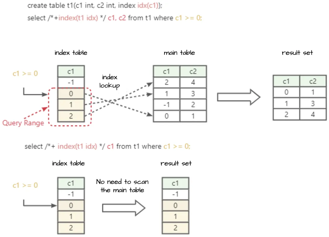
Scan less data when you query a specified column

Assume that a wide rowstore table contains 100 columns. If you need to frequently access one of the columns, we recommend that you create an index on the column. An index generally contains a few columns, which can avoid full table scans. However, indexes are not required when you query a few columns of a wide columnstore table in OceanBase Database.

In the plan for the following statement, the value of NAME is test(idx_b), which indicates that the index idx_b is used in the query. This way, data of the a, c, and d columns does not need to be scanned.

create table test(a int, b int, c int, d int, key idx_b(b));

explain select b from test;
+---------------------------------------------------------------------------------------+
| Query Plan                                                                            |
+---------------------------------------------------------------------------------------+
| ======================================================                                |
| |ID|OPERATOR       |NAME       |EST.ROWS|EST.TIME(us)|                                |
| ------------------------------------------------------                                |
| |0 |TABLE FULL SCAN|test(idx_b)|1       |2           |                                |
| ======================================================                                |
| Outputs & filters:                                                                    |
| -------------------------------------                                                 |
|   0 - output([test.b]), filter(nil), rowset=256                                       |
|       access([test.b]), partitions(p0)                                                |
|       is_index_back=false, is_global_index=false,                                     |
|       range_key([test.b], [test. __pk_increment]), range(MIN,MIN ; MAX,MAX)always true |
+---------------------------------------------------------------------------------------+
11 rows in set

The plan for the following statement shows that the optimizer will scan the index idx_b that contains the fewest columns, namely containing the smallest amount of data.

create table test(a int, b int, c int, d int, key idx_b(b));

explain select count(*) from test;
+-----------------------------------------------------------------------------------------+
| Query Plan                                                                              |
+-----------------------------------------------------------------------------------------+
| ========================================================                                |
| |ID|OPERATOR         |NAME       |EST.ROWS|EST.TIME(us)|                                |
| --------------------------------------------------------                                |
| |0 |SCALAR GROUP BY  |           |1       |2           |                                |
| |1 |└─TABLE FULL SCAN|test(idx_b)|1       |2           |                                |
| ========================================================                                |
| Outputs & filters:                                                                      |
| -------------------------------------                                                   |
|   0 - output([T_FUN_COUNT_SUM(T_FUN_COUNT(*))]), filter(nil), rowset=256                |
|       group(nil), agg_func([T_FUN_COUNT_SUM(T_FUN_COUNT(*))])                           |
|   1 - output([T_FUN_COUNT(*)]), filter(nil), rowset=256                                 |
|       access(nil), partitions(p0)                                                       |
|       is_index_back=false, is_global_index=false,                                       |
|       range_key([test.b], [test. __pk_increment]), range(MIN,MIN ; MAX,MAX)always true,  |
|       pushdown_aggregation([T_FUN_COUNT(*)])                                            |
+-----------------------------------------------------------------------------------------+

However, if you use an index when you query a large number of columns, table access by index primary key is required. You must query other columns from the primary table based on the primary key column contained in the index. The cost of table access by index primary key is very high. Generally, the performance of table access by index primary key is only 1/10 that of a full table scan. Especially, if the filter condition has poor selectivity, the cost of table access by index primary key is impossible to ignore.

The following statement queries all rows of the a and b columns, with an index created on the b column. The EST.TIME value estimated by the optimizer for a full table scan without using the index is 2 µs.

create table test(a int, b int, c int, d int, key idx_b(b));

explain select a, b from test;
+---------------------------------------------------------------------+
| Query Plan                                                          |
+---------------------------------------------------------------------+
| ===============================================                     |
| |ID|OPERATOR       |NAME|EST.ROWS|EST.TIME(us)|                     |
| -----------------------------------------------                     |
| |0 |TABLE FULL SCAN|test|1       |2           |                     |
| ===============================================                     |
| Outputs & filters:                                                  |
| -------------------------------------                               |
|   0 - output([test.a], [test.b]), filter(nil), rowset=256           |
|       access([test.a], [test.b]), partitions(p0)                    |
|       is_index_back=false, is_global_index=false,                   |
|       range_key([test. __pk_increment]), range(MIN ; MAX)always true |
+---------------------------------------------------------------------+

In the following statement, the hint specifies to use the index, and the EST.TIME value estimated by the optimizer for the query is 5 µs, which is longer than that of a full table scan. This is because table access by index primary key (is_index_back=true) causes additional overheads.

explain select /*+ index(test idx_b) */ a, b from test;

The output is as follows:

+---------------------------------------------------------------------------------------+
| Query Plan                                                                            |
+---------------------------------------------------------------------------------------+
| ======================================================                                |
| |ID|OPERATOR       |NAME       |EST.ROWS|EST.TIME(us)|                                |
| ------------------------------------------------------                                |
| |0 |TABLE FULL SCAN|test(idx_b)|1       |5           |                                |
| ======================================================                                |
| Outputs & filters:                                                                    |
| -------------------------------------                                                 |
|   0 - output([test.a], [test.b]), filter(nil), rowset=256                             |
|       access([test. __pk_increment], [test.a], [test.b]), partitions(p0)               |
|       is_index_back=true, is_global_index=false,                                      |
|       range_key([test.b], [test. __pk_increment]), range(MIN,MIN ; MAX,MAX)always true |
+---------------------------------------------------------------------------------------+

Measure the overhead of an index

The overhead of an index contains two parts:

1. The amount of time taken to scan the index, which depends on the number of data rows scanned

2. The amount of time taken to access the primary table by index primary key, which depends on the number of data rows to be accessed by index primary key

Assume that a table contains 10,000 rows of data, the amount of time taken to scan an index is 1 ms per 1,000 rows, and the amount of time taken to access the primary table by index primary key is 1 ms per 100 rows, which is approximately 10 times that to scan the index.

create table test(a int primary key, b int, c int, d int, e int, key idx_b_e_c(b, e, c));

The filter condition b = 1 and c = 1 can return 1,000 rows of data.

Assume that you need to execute the select a, b, c from test where b = 1 and c = 1; statement. If you use the index, the execution overhead is 1 ms, which is the amount of time taken to scan the 1,000 rows of data in the index.

explain select /*+index(test idx_b_c_d)*/ a, b, c from test where b = 1 and c = 1;

If you do not use the index, the execution overhead is 10 ms, which is the amount of time taken to scan the 10,000 rows of data in the primary table.

explain select /*+index(test primary)*/ a, b, c from test where b = 1 and c = 1;

In this scenario, the query with the index used is faster. If the generated plan contains no index, you can use the hint /*+index(test idx_b_c_d)*/ to specify to use an index.

Assume that you need to execute the select * from test where b = 1 and c = 1; statement. If you use the index idx_b_c_d, the execution overhead is 11 ms, which is equal to 1 ms + 10 ms. 1 ms is the amount of time taken to scan the 1,000 rows of data in the index, and 10 ms is the amount of time taken to scan 1,000 rows of data in the primary table by index primary key.

explain select /*+index(test idx_b_c_d)*/ * from test where b = 1 and c = 1;

If you do not use the index, the execution overhead is 10 ms, which is the amount of time taken to scan the 10,000 rows of data in the primary table.

explain select /*+index(test primary)*/ * from test where b = 1 and c = 1;

In this scenario, the query without using the index is faster. If the generated plan contains an index, you can use the hint /*+index(test primary)*/ to specify to access the primary table without using the index.

If you want to know the number of rows returned when you use the filter condition b = 1 and c = 1, execute the following SQL statement and check the count value in the output.

select count(*) from test where b = 1 and c = 1;

The output is as follows:

+----------+
| count(*) |
+----------+
|      1000|
+----------+

Summary

Observe the following strategies when you create an index:

• In a common query, place a column with an equality condition before an index and a column with a range condition after the index.

• If a common query involves multiple columns with range conditions, create an index on the column with higher selectivity.

• Create a covering index on multiple columns to avoid access to the primary table.

Assume that an SQL statement contains three filter conditions: a = 1, b > 0, and c between 1 and 12, where b > 0 can filter out 30% of the data, and c between 1 and 12 can filter out 90% of the data. According to the preceding strategies, you can create an index on the (a, c, b) columns to optimize this statement.

Columns a and c are the first two columns in the index. Column b is added to the end of the index to avoid access to the primary table when column b is selected in the query.

Access to the primary table causes additional overheads. In some extreme scenarios, we may encounter a query that does not read many rows in a single execution but still leads to a very large number of data reads on the whole due to its high queries per second (QPS) value. If the I/O capacity of a server is limited, the disk I/O may be used up. Here is an example:

-- Create a wide table with 4,000 columns.
CREATE TABLE T1 (C1 INT, C2 INT, C3 INT, C4 INT, ... , C4000 INT);

CREATE INDEX IDX_C1 ON T1 (C1);

EXPLAIN SELECT C3, C4 FROM T1 WHERE C1 = 1;
+-----------------------------------------------------------------------+
| Query Plan                                                            |
+-----------------------------------------------------------------------+
| ======================================================                |
| |ID|OPERATOR        |NAME      |EST.ROWS|EST.TIME(us)|                |
| ------------------------------------------------------                |
| |0 |TABLE RANGE SCAN|t1(IDX_C1)|1       |7           |                |
| ======================================================                |
| Outputs & filters:                                                    |
| -------------------------------------                                 |
|   0 - output([t1.C3], [t1.C4]), filter(nil), rowset=16                |
|       access([t1.__pk_increment], [t1.C3], [t1.C4]), partitions(p0)   |
|       is_index_back=true, is_global_index=false,                      |
|       range_key([t1.C1], [t1.__pk_increment]), range(1,MIN ; 1,MAX),  |
|       range_cond([t1.C1 = 1])                                         |
+-----------------------------------------------------------------------+

After the preceding query uses the index on the C1 column, the optimal query range is obtained. The query scans a small amount of data on the index IDX_C1 each time.

However, the query needs to get values in the C3 and C4 columns but the index IDX_C1 does not contain the values of these two columns, so the query still needs to get the values from the primary table by index primary key (is_index_back=true). Each query execution involves a small number of sequential reads on the index IDX_C1 and a small number of random reads on the primary table. When the QPS value of the query becomes very high, a large number of random reads may be performed on the primary table, which consumes a large amount of system I/O resources.

In this case, you may create a covering index to avoid access to the primary table. Taking the preceding query as an example, you can create a covering index as follows:

CREATE INDEX IDX_C1_C3_C4 ON T1 (C1, C3, C4);

EXPLAIN SELECT C3, C4 FROM T1 WHERE C1 = 1;
+---------------------------------------------------------------------------------------------------------+
| Query Plan                                                                                              |
+---------------------------------------------------------------------------------------------------------+
| ============================================================                                            |
| |ID|OPERATOR        |NAME            |EST.ROWS|EST.TIME(us)|                                            |
| ------------------------------------------------------------                                            |
| |0 |TABLE RANGE SCAN|t1(IDX_C1_C3_C4)|1       |4           |                                            |
| ============================================================                                            |
| Outputs & filters:                                                                                      |
| -------------------------------------                                                                   |
|   0 - output([t1.C3], [t1.C4]), filter(nil), rowset=16                                                  |
|       access([t1.C3], [t1.C4]), partitions(p0)                                                          |
|       is_index_back=false, is_global_index=false,                                                       |
|       range_key([t1.C1], [t1.C3], [t1.C4], [t1.__pk_increment]), range(1,MIN,MIN,MIN ; 1,MAX,MAX,MAX),  |
|       range_cond([t1.C1 = 1])                                                                           |
+---------------------------------------------------------------------------------------------------------+

When the query accesses the index IDX_C1_C3_C4, it reads data in the optimal query range without the need to access the primary table (is_index_back=false). When the query is executed, only a small number of sequential scans are performed on the index. This greatly reduces the I/O resource usage.

Generally, you need to create a covering index in scenarios with the following characteristics:

• The I/O pressure on the database is very high.

• The high I/O is mainly caused by random I/O for accessing the primary table in queries with high QPS values.

• Queries with high QPS values actually do not need to read data from many columns.

In such scenarios, you can create covering indexes for the queries with high QPS values to optimize their execution.

Note

The preceding three strategies are not omnipotent and must be used in consideration of specific tuning scenarios.

Join tuning

Index tuning is the most basic method for SQL performance tuning.

Join tuning is more complex than index tuning. This section briefly describes several join algorithms without in-depth discussion.

OceanBase Database supports three basic join algorithms: NESTED-LOOP JOIN, MERGE JOIN, and HASH JOIN.

• NESTED-LOOP JOIN: scans the data on the left of the join operator, and then uses each row in the left-side table to traverse the data in the right-side table to find all data rows that can be joined. Cost of the join = Cost of scanning the left-side table + Number of rows in the left-side table × Cost of using each row in the left-side table to traverse the right-side table, that is, cost(NLJ) = cost(left) + N(left) * cost(right). The time complexity is O(m * n).

• MERGE JOIN (also called SORT-MERGE JOIN): sorts the join keys in the left-side and right-side tables separately, and then continuously adjusts the pointer, for example, moves the pointer, to find matching rows to join. Cost of the join = Costs of sorting the left-side and right-side tables + Costs of scanning the left-side and right-side tables, that is, cost(MJ) = sort(left) + sort(right) + cost(left) + cost(right). The time complexity is O(n * logn), which is also the time complexity of sorting.

• HASH JOIN: scans the left-side table and creates a hash table for each row, and then scans the right-side table and probes the hash tables to match and join rows. Cost of the join = Cost of scanning the left-side table + Number of rows in the left-side table × Cost of creating a hash table for each row + Cost of scanning the right-side table + Number of rows in the right-side table × Cost of probing the hash table for each row, that is, cost(HJ) = cost(left) + N(left) * create_hash_cost + cost(right) + N(right) * probe_hash_cost.

NESTED-LOOP JOIN

OceanBase Database supports nested-loop joins with and without condition pushdown.

These two types of nested-loop joins cause different overheads. Before you perform a nested-loop join, create two tables named t1 and t2, use recursive cte to insert 1,000 rows of data into each table, and then use the dbms_stats.gather_table_stats function to collect statistics.

drop table t1;

drop table t2;

CREATE TABLE t1
WITH RECURSIVE my_cte(a, b, c) AS
(
  SELECT 1, 0, 0
  UNION ALL
  SELECT a + 1, round((a + 1) / 2, 0), round((a + 1) / 3, 0) FROM my_cte WHERE a < 1000
)
SELECT * FROM my_cte;

alter table t1 add primary key(a);

CREATE TABLE t2
WITH RECURSIVE my_cte(a, b, c) AS
(
  SELECT 1, 0, 0
  UNION ALL
  SELECT a + 1, round((a + 1) / 2, 0), round((a + 1) / 3, 0) FROM my_cte WHERE a < 1000
)
SELECT * FROM my_cte;

alter table t2 add primary key(a);

call dbms_stats.gather_table_stats('TEST', 'T1', method_opt=>'for all columns size auto', estimate_percent=>100);

call dbms_stats.gather_table_stats('TEST', 'T2', method_opt=>'for all columns size auto', estimate_percent=>100);

Nested-loop join without condition pushdown

You can use the hint /*+ leading(t1 t2) use_nl(t1, t2)*/ to specify to generate a nested-loop join plan for the following statement. The t2 table has no suitable index and the b column is not a primary key column. Therefore, all data of the t2 table must be scanned and then the MATERIAL operator is used to materialize the data into memory. In this case, all rows of the t2 table must be traversed upon access to each row of the t1 table. This is equivalent to calculating a Cartesian product with the time complexity being O(m * n), leading to poor performance.

Theoretically, execution plans not controlled by hints or outlines contain only the NESTED-LOOP JOIN operator with condition pushdown.

explain select /*+ leading(t1 t2) use_nl(t1, t2)*/ * from t1, t2 where t1.b = t2.b;

The output is as follows:

+---------------------------------------------------------------------------------------+
| Query Plan                                                                            |
+---------------------------------------------------------------------------------------+
| ===================================================                                   |
| |ID|OPERATOR           |NAME|EST.ROWS|EST.TIME(us)|                                   |
| ---------------------------------------------------                                   |
| |0 |NESTED-LOOP JOIN   |    |1877    |11578       |                                   |
| |1 |├─TABLE FULL SCAN  |t1  |1000    |84          |                                   |
| |2 |└─MATERIAL         |    |1000    |179         |                                   |
| |3 |  └─TABLE FULL SCAN|t2  |1000    |84          |                                   |
| ===================================================                                   |
| Outputs & filters:                                                                    |
| -------------------------------------                                                 |
|   0 - output([t1.a], [t1.b], [t1.c], [t2.a], [t2.b], [t2.c]), filter(nil), rowset=256 |
|       conds([t1.b = t2.b]), nl_params_(nil), use_batch=false                          |
|   1 - output([t1.a], [t1.b], [t1.c]), filter(nil), rowset=256                         |
|       access([t1.a], [t1.b], [t1.c]), partitions(p0)                                  |
|       is_index_back=false, is_global_index=false,                                     |
|       range_key([t1.a]), range(MIN ; MAX)always true                                  |
|   2 - output([t2.a], [t2.b], [t2.c]), filter(nil), rowset=256                         |
|   3 - output([t2.a], [t2.b], [t2.c]), filter(nil), rowset=256                         |
|       access([t2.a], [t2.b], [t2.c]), partitions(p0)                                  |
|       is_index_back=false, is_global_index=false,                                     |
|       range_key([t2.a]), range(MIN ; MAX)always true                                  |
+---------------------------------------------------------------------------------------+
21 rows in set

Nested-loop join with condition pushdown

You can change the join condition to t1.a = t2.a and use the hint /*+ leading(t1 t2) use_nl(t1, t2)*/ to specify to generate a nested-loop join plan for the following statement.

The nl_params field in the plan contains t1.a. Therefore, the query first scans the t1 table on the left of the join operator and then uses the a value of each row of the t1 table as a filter condition to get data from the right-side table. The TABLE GET operator gets data from the right-side table by primary key based on the range condition t1.a = t2.a. The t2 table on the right has a primary key on the a column. Therefore, the TABLE GET operator can directly obtain any specific value. The time complexity is only O(m).

explain select /*+ leading(t1 t2) use_nl(t1, t2)*/ * from t1, t2 where t1.a = t2.a;

The output is as follows:

+---------------------------------------------------------------------------------------+
| Query Plan                                                                            |
+---------------------------------------------------------------------------------------+
| =======================================================                               |
| |ID|OPERATOR               |NAME|EST.ROWS|EST.TIME(us)|                               |
| -------------------------------------------------------                               |
| |0 |NESTED-LOOP JOIN       |    |1000    |16274       |                               |
| |1 |├─TABLE FULL SCAN      |t1  |1000    |84          |                               |
| |2 |└─DISTRIBUTED TABLE GET|t2  |1       |16          |                               |
| =======================================================                               |
| Outputs & filters:                                                                    |
| -------------------------------------                                                 |
|   0 - output([t1.a], [t1.b], [t1.c], [t2.a], [t2.b], [t2.c]), filter(nil), rowset=256 |
|       conds(nil), nl_params_([t1.a(:0)]), use_batch=true                              |
|   1 - output([t1.a], [t1.b], [t1.c]), filter(nil), rowset=256                         |
|       access([t1.a], [t1.b], [t1.c]), partitions(p0)                                  |
|       is_index_back=false, is_global_index=false,                                     |
|       range_key([t1.a]), range(MIN ; MAX)always true                                  |
|   2 - output([t2.a], [t2.b], [t2.c]), filter(nil), rowset=256                         |
|       access([GROUP_ID], [t2.a], [t2.b], [t2.c]), partitions(p0)                      |
|       is_index_back=false, is_global_index=false,                                     |
|       range_key([t2.a]), range(MIN ; MAX),                                            |
|       range_cond([:0 = t2.a])                                                         |
+---------------------------------------------------------------------------------------+

In OceanBase Database, the NESTED-LOOP JOIN operator with condition pushdown is generally used. The NESTED-LOOP JOIN operator without condition pushdown may be used only in the absence of an equality join condition or appropriate index. However, in this case, the HASH JOIN or MERGE JOIN operator is more likely to be used instead. If a plan contains the NESTED-LOOP JOIN operator without condition pushdown, carefully check whether it is appropriate.

SUBPLAN FILTER

Like the NESTED-LOOP JOIN operator, the SUBPLAN FILTER operator also requires an appropriate index or primary key for condition pushdown.

The t1 and t2 tables with their primary keys created on the a columns are still used as an example here. The plan generated for the following statement contains the SUBPLAN FILTER operator in the absence of an appropriate index or primary key. The performance of the SUBPLAN FILTER operator is almost the same as that of the NESTED-LOOP JOIN operator without condition pushdown.

explain select /*+no_rewrite*/ a from t1 where b > (select b from t2 where t1.b = t2.b);

The output is as follows:

+--------------------------------------------------------------------------------------------+
| Query Plan                                                                                 |
+--------------------------------------------------------------------------------------------+
| =================================================                                          |
| |ID|OPERATOR         |NAME|EST.ROWS|EST.TIME(us)|                                          |
| -------------------------------------------------                                          |
| |0 |SUBPLAN FILTER   |    |334     |45415       |                                          |
| |1 |├─TABLE FULL SCAN|t1  |1000    |60          |                                          |
| |2 |└─TABLE FULL SCAN|t2  |2       |46          |                                          |
| =================================================                                          |
| Outputs & filters:                                                                         |
| -------------------------------------                                                      |
|   0 - output([t1.a]), filter([t1.b > subquery(1)]), rowset=256                             |
|       exec_params_([t1.b(:0)]), onetime_exprs_(nil), init_plan_idxs_(nil), use_batch=false |
|   1 - output([t1.a], [t1.b]), filter(nil), rowset=256                                      |
|       access([t1.a], [t1.b]), partitions(p0)                                               |
|       is_index_back=false, is_global_index=false,                                          |
|       range_key([t1.a]), range(MIN ; MAX)always true                                       |
|   2 - output([t2.b]), filter([:0 = t2.b]), rowset=256                                      |
|       access([t2.b]), partitions(p0)                                                       |
|       is_index_back=false, is_global_index=false, filter_before_indexback[false],          |
|       range_key([t2.a]), range(MIN ; MAX)always true                                       |
+--------------------------------------------------------------------------------------------+

The plan generated for the following statement contains the SUBPLAN FILTER operator in the presence an appropriate primary key. The performance of the SUBPLAN FILTER operator is almost the same as that of the NESTED-LOOP JOIN operator with condition pushdown.

explain select /*+no_rewrite*/ a from t1 where b > (select b from t2 where t1.a = t2.a);

The output is as follows:

+-------------------------------------------------------------------------------------------+
| Query Plan                                                                                |
+-------------------------------------------------------------------------------------------+
| =======================================================                                   |
| |ID|OPERATOR               |NAME|EST.ROWS|EST.TIME(us)|                                   |
| -------------------------------------------------------                                   |
| |0 |SUBPLAN FILTER         |    |334     |18043       |                                   |
| |1 |├─TABLE FULL SCAN      |t1  |1000    |60          |                                   |
| |2 |└─DISTRIBUTED TABLE GET|t2  |1       |18          |                                   |
| =======================================================                                   |
| Outputs & filters:                                                                        |
| -------------------------------------                                                     |
|   0 - output([t1.a]), filter([t1.b > subquery(1)]), rowset=256                            |
|       exec_params_([t1.a(:0)]), onetime_exprs_(nil), init_plan_idxs_(nil), use_batch=true |
|   1 - output([t1.a], [t1.b]), filter(nil), rowset=256                                     |
|       access([t1.a], [t1.b]), partitions(p0)                                              |
|       is_index_back=false, is_global_index=false,                                         |
|       range_key([t1.a]), range(MIN ; MAX)always true                                      |
|   2 - output([t2.b]), filter(nil), rowset=256                                             |
|       access([GROUP_ID], [t2.b]), partitions(p0)                                          |
|       is_index_back=false, is_global_index=false,                                         |
|       range_key([t2.a]), range(MIN ; MAX)always true,                                     |
|       range_cond([:0 = t2.a])                                                             |
+-------------------------------------------------------------------------------------------+

In OceanBase Database, not all subqueries can be unnested. Some SQL queries can use only the SUBPLAN FILTER operator based on their semantics. The execution of the SUBPLAN FILTER operator is similar to that of the NESTED-LOOP JOIN operator. Therefore, an appropriate index is required to avoid using the SUBPLAN FILTER operator without condition pushdown.

HASH JOIN

• cost(NLJ) = cost(left) + N(left) * cost(right)

• cost(HJ) = cost(left) + N(left) * create_hash_cost + cost(right) + N(right) * probe_hash_cost

The preceding formulas calculate the costs of the NESTED-LOOP JOIN and HASH JOIN operators respectively. The optimizer selects the NESTED-LOOP JOIN operator only under the following two conditions:

1. The right-side table has an appropriate index or primary key.

2. The number of rows in the left-side or right-side table exceeds a specified threshold, which is approximately 20 in OceanBase Database.

Here is an example: Create two tables named t1 and t2, where the t1 table has no primary key and contains 10 rows, and the t2 table has a primary key on the a column and contains 1,000 rows.

drop table t1;

drop table t2;

CREATE TABLE t1
WITH RECURSIVE my_cte(a, b, c) AS
(
  SELECT 1, 0, 0
  UNION ALL
  SELECT a + 1, round((a + 1) / 2, 0), round((a + 1) / 3, 0) FROM my_cte WHERE a < 10
)
SELECT * FROM my_cte;

CREATE TABLE t2
WITH RECURSIVE my_cte(a, b, c) AS
(
  SELECT 1, 0, 0
  UNION ALL
  SELECT a + 1, round((a + 1) / 2, 0), round((a + 1) / 3, 0) FROM my_cte WHERE a < 1000
)
SELECT * FROM my_cte;

alter table t2 add primary key(a);

call dbms_stats.gather_table_stats('TEST', 'T1', method_opt=>'for all columns size auto', estimate_percent=>100);

call dbms_stats.gather_table_stats('TEST', 'T2', method_opt=>'for all columns size auto', estimate_percent=>100);

In the following statement, the primary key of the t2 table is not used in table access, so a hash join plan is generated instead of a nested-loop join plan. This is because only a nested-loop join plan without condition pushdown can be generated in this scenario, which has a high cost.

explain select * from t1, t2 where t1.b = t2.b;

The output is as follows:

+---------------------------------------------------------------------------------------+
| Query Plan                                                                            |
+---------------------------------------------------------------------------------------+
| =================================================                                     |
| |ID|OPERATOR         |NAME|EST.ROWS|EST.TIME(us)|                                     |
| -------------------------------------------------                                     |
| |0 |HASH JOIN        |    |1       |4           |                                     |
| |1 |├─TABLE FULL SCAN|t1  |1       |2           |                                     |
| |2 |└─TABLE FULL SCAN|t2  |1       |2           |                                     |
| =================================================                                     |
| Outputs & filters:                                                                    |
| -------------------------------------                                                 |
|   0 - output([t1.a], [t1.b], [t1.c], [t2.a], [t2.b], [t2.c]), filter(nil), rowset=256 |
|       equal_conds([t1.b = t2.b]), other_conds(nil)                                    |
|   1 - output([t1.a], [t1.b], [t1.c]), filter(nil), rowset=256                         |
|       access([t1.a], [t1.b], [t1.c]), partitions(p0)                                  |
|       is_index_back=false, is_global_index=false,                                     |
|       range_key([t1.a]), range(MIN ; MAX)always true                                  |
|   2 - output([t2.b], [t2.a], [t2.c]), filter(nil), rowset=256                         |
|       access([t2.b], [t2.a], [t2.c]), partitions(p0)                                  |
|       is_index_back=false, is_global_index=false,                                     |
|       range_key([t2.__pk_increment]), range(MIN ; MAX)always true                     |
+---------------------------------------------------------------------------------------+

In the following statement, the primary key column t2.a of the t2 table is used in table access, and the number of rows in the t2 table on the right greatly differs from that in the t1 table on the left. Therefore, a nested-loop join plan is generated.

explain select * from t1, t2 where t1.a = t2.a;

The output is as follows:

+---------------------------------------------------------------------------------------+
| Query Plan                                                                            |
+---------------------------------------------------------------------------------------+
| =======================================================                               |
| |ID|OPERATOR               |NAME|EST.ROWS|EST.TIME(us)|                               |
| -------------------------------------------------------                               |
| |0 |NESTED-LOOP JOIN       |    |10      |165         |                               |
| |1 |├─TABLE FULL SCAN      |t1  |10      |3           |                               |
| |2 |└─DISTRIBUTED TABLE GET|t2  |1       |16          |                               |
| =======================================================                               |
| Outputs & filters:                                                                    |
| -------------------------------------                                                 |
|   0 - output([t1.a], [t1.b], [t1.c], [t2.a], [t2.b], [t2.c]), filter(nil), rowset=256 |
|       conds(nil), nl_params_([t1.a(:0)]), use_batch=true                              |
|   1 - output([t1.a], [t1.b], [t1.c]), filter(nil), rowset=256                         |
|       access([t1.a], [t1.b], [t1.c]), partitions(p0)                                  |
|       is_index_back=false, is_global_index=false,                                     |
|       range_key([t1.__pk_increment]), range(MIN ; MAX)always true                     |
|   2 - output([t2.a], [t2.b], [t2.c]), filter(nil), rowset=256                         |
|       access([GROUP_ID], [t2.a], [t2.b], [t2.c]), partitions(p0)                      |
|       is_index_back=false, is_global_index=false,                                     |
|       range_key([t2.a]), range(MIN ; MAX),                                            |
|       range_cond([:0 = t2.a])                                                         |
+---------------------------------------------------------------------------------------+

MERGE JOIN

• cost(MJ) = cost(left) + cost(right) + sort(left) + sort(right)

• cost(HJ) = cost(left) + N(left) * hash_cost + cost(right) + N(right) * probe_cost

The preceding formulas calculate the costs of the MERGE JOIN and HASH JOIN operators respectively. Both operators must fully scan the left-side and right-side tables. However, the MERGE JOIN operator sorts the join keys in both tables separately, and the HASH JOIN operator creates hash tables for the left-side table and probes hash tables for the right-side table. The cost O(n) of creating and probing hash tables is lower than the cost O(nlogn) of sorting. Therefore, the HASH JOIN operator is generally superior to the MERGE JOIN operator.

The MERGE JOIN operator is used only in special scenarios. For example, when both the left-side and right-side tables are ordered, the MERGE JOIN operator is used because it performs only a merge without sorting.

The t1 and t2 tables with their primary keys created on the a columns are still used as an example here.

drop table t1;

drop table t2;

CREATE TABLE t1
WITH RECURSIVE my_cte(a, b, c) AS
(
  SELECT 1, 0, 0
  UNION ALL
  SELECT a + 1, round((a + 1) / 2, 0), round((a + 1) / 3, 0) FROM my_cte WHERE a < 1000
)
SELECT * FROM my_cte;

alter table t1 add primary key(a);

CREATE TABLE t2
WITH RECURSIVE my_cte(a, b, c) AS
(
  SELECT 1, 0, 0
  UNION ALL
  SELECT a + 1, round((a + 1) / 2, 0), round((a + 1) / 3, 0) FROM my_cte WHERE a < 1000
)
SELECT * FROM my_cte;

alter table t2 add primary key(a);

call dbms_stats.gather_table_stats('TEST', 'T1', method_opt=>'for all columns size auto', estimate_percent=>100);

call dbms_stats.gather_table_stats('TEST', 'T2', method_opt=>'for all columns size auto', estimate_percent=>100);

In the following statement, the join condition is the ordered primary key columns a of both tables, so a merge join plan is generated.

explain select * from t1, t2 where t1.a = t2.a;
+---------------------------------------------------------------------------------------+
| Query Plan                                                                            |
+---------------------------------------------------------------------------------------+
| =================================================                                     |
| |ID|OPERATOR         |NAME|EST.ROWS|EST.TIME(us)|                                     |
| -------------------------------------------------                                     |
| |0 |MERGE JOIN       |    |1000    |301         |                                     |
| |1 |├─TABLE FULL SCAN|t1  |1000    |84          |                                     |
| |2 |└─TABLE FULL SCAN|t2  |1000    |84          |                                     |
| =================================================                                     |
| Outputs & filters:                                                                    |
| -------------------------------------                                                 |
|   0 - output([t1.a], [t1.b], [t1.c], [t2.a], [t2.b], [t2.c]), filter(nil), rowset=256 |
|       equal_conds([t1.a = t2.a]), other_conds(nil)                                    |
|       merge_directions([ASC])                                                         |
|   1 - output([t1.a], [t1.b], [t1.c]), filter(nil), rowset=256                         |
|       access([t1.a], [t1.b], [t1.c]), partitions(p0)                                  |
|       is_index_back=false, is_global_index=false,                                     |
|       range_key([t1.a]), range(MIN ; MAX)always true                                  |
|   2 - output([t2.a], [t2.b], [t2.c]), filter(nil), rowset=256                         |
|       access([t2.a], [t2.b], [t2.c]), partitions(p0)                                  |
|       is_index_back=false, is_global_index=false,                                     |
|       range_key([t2.a]), range(MIN ; MAX)always true                                  |
+---------------------------------------------------------------------------------------+

In the following statement, the join condition is the unordered b columns of both tables, so a hash join plan is generated.

explain select * from t1, t2 where t1.b = t2.b;

The output is as follows:

+---------------------------------------------------------------------------------------+
| Query Plan                                                                            |
+---------------------------------------------------------------------------------------+
| =================================================                                     |
| |ID|OPERATOR         |NAME|EST.ROWS|EST.TIME(us)|                                     |
| -------------------------------------------------                                     |
| |0 |HASH JOIN        |    |1877    |481         |                                     |
| |1 |├─TABLE FULL SCAN|t1  |1000    |84          |                                     |
| |2 |└─TABLE FULL SCAN|t2  |1000    |84          |                                     |
| =================================================                                     |
| Outputs & filters:                                                                    |
| -------------------------------------                                                 |
|   0 - output([t1.a], [t1.b], [t1.c], [t2.a], [t2.b], [t2.c]), filter(nil), rowset=256 |
|       equal_conds([t1.b = t2.b]), other_conds(nil)                                    |
|   1 - output([t1.a], [t1.b], [t1.c]), filter(nil), rowset=256                         |
|       access([t1.a], [t1.b], [t1.c]), partitions(p0)                                  |
|       is_index_back=false, is_global_index=false,                                     |
|       range_key([t1.a]), range(MIN ; MAX)always true                                  |
|   2 - output([t2.a], [t2.b], [t2.c]), filter(nil), rowset=256                         |
|       access([t2.a], [t2.b], [t2.c]), partitions(p0)                                  |
|       is_index_back=false, is_global_index=false,                                     |
|       range_key([t2.a]), range(MIN ; MAX)always true                                  |
+---------------------------------------------------------------------------------------+

In the following statement, the join condition is the unordered b columns of both tables, and the hint specifies to generate a merge join plan, so a merge join plan with the SORT operator is generated. In this plan, a merge join is performed after sorting, and the cost is higher than that of a hash join plan.

explain select /*+ USE_MERGE(t1 t2) */ * from t1, t2 where t1.b = t2.b;

The output is as follows:

+---------------------------------------------------------------------------------------+
| Query Plan                                                                            |
+---------------------------------------------------------------------------------------+
| ===================================================                                   |
| |ID|OPERATOR           |NAME|EST.ROWS|EST.TIME(us)|                                   |
| ---------------------------------------------------                                   |
| |0 |MERGE JOIN         |    |1877    |750         |                                   |
| |1 |├─SORT             |    |1000    |294         |                                   |
| |2 |│ └─TABLE FULL SCAN|t1  |1000    |84          |                                   |
| |3 |└─SORT             |    |1000    |294         |                                   |
| |4 |  └─TABLE FULL SCAN|t2  |1000    |84          |                                   |
| ===================================================                                   |
| Outputs & filters:                                                                    |
| -------------------------------------                                                 |
|   0 - output([t1.a], [t1.b], [t1.c], [t2.a], [t2.b], [t2.c]), filter(nil), rowset=256 |
|       equal_conds([t1.b = t2.b]), other_conds(nil)                                    |
|       merge_directions([ASC])                                                         |
|   1 - output([t1.a], [t1.b], [t1.c]), filter(nil), rowset=256                         |
|       sort_keys([t1.b, ASC])                                                          |
|   2 - output([t1.a], [t1.b], [t1.c]), filter(nil), rowset=256                         |
|       access([t1.a], [t1.b], [t1.c]), partitions(p0)                                  |
|       is_index_back=false, is_global_index=false,                                     |
|       range_key([t1.a]), range(MIN ; MAX)always true                                  |
|   3 - output([t2.a], [t2.b], [t2.c]), filter(nil), rowset=256                         |
|       sort_keys([t2.b, ASC])                                                          |
|   4 - output([t2.a], [t2.b], [t2.c]), filter(nil), rowset=256                         |
|       access([t2.a], [t2.b], [t2.c]), partitions(p0)                                  |
|       is_index_back=false, is_global_index=false,                                     |
|       range_key([t2.a]), range(MIN ; MAX)always true                                  |
+---------------------------------------------------------------------------------------+

Summary

These three join methods are commonly used in databases. Note that:

• Most plans use the NESTED-LOOP JOIN operator with condition pushdown. If a plan uses the NESTED-LOOP JOIN operator without condition pushdown, you must create an appropriate index to change it to NESTED-LOOP JOIN with condition pushdown or use a hint to specify to use another join method. For more information about the hints related to joins, see Hints related to joins.

• The execution of the SUBPLAN FILTER operator is similar to that of the NESTED-LOOP JOIN operator. Therefore, an appropriate index is also required to avoid using a SUBPLAN FILTER operator without condition pushdown.

• If a plan contains the MERGE JOIN operator, subsequent operators are expected to be ordered. If not, SORT operators are required for sorting before the merge. In this case, you can use a hint to change the join method to HASH JOIN as needed.

• If you want to join unordered data without an appropriate index or primary key, HASH JOIN generally has the lowest cost.

ORDER BY and LIMIT tuning

The ORDER BY and LIMIT clauses are commonly used in business queries to obtain a sorted result set that contains a specified number of rows. To return such a result set, an efficient execution plan generated by the optimizer may need to read only a small amount of data from target tables, but an inefficient plan may need to read all the data. For the purpose of optimization, you must first understand why the optimizer generates two types of execution plans, and then try to obtain the efficient one.

Optimize SORT generation

When a query contains a LIMIT clause, the execution performance highly depends on whether the generated execution plan contains a blocking operator. A blocking operator requires a query to obtain all rows of subnodes before it returns rows to the parent node. SORT is a common blocking operator. When a query contains an ORDER BY clause or an operator that depends on sorting, such as MERGE DISTINCT, MERGE GROUP BY, or MERGE JOIN, needs to be assigned to the generated plan, the optimizer tries to assign the SORT operator to obtain the intermediate result set sorted by the specified keys. To avoid assigning unnecessary SORT operators and make full use of existing sorted intermediate result sets, the optimizer maintains some sort-related information and performs optimization when it tries to assign a SORT operator.

Order in a plan tree

In an execution plan, the input of an operator may be sorted. For base table scans, the order comes from indexed columns. For other operators, this order may come from the output order of child operators. Different from the output order explicitly required by ORDER BY, the input order required by most operators that depend on sorting are adjustable, and can be inherited by the output of the operators. By optimizing the order used for operators that depend on sorting, the optimizer can avoid unnecessary sorts.

When the optimizer determines the order for an operator that depends on sorting, it checks the existing input order and the order that may be required later. For example, in the following query, a MERGE GROUP BY operator is assigned for the GROUP BY clause, and the optimizer can swap the positions of c1 and c2 and change the sorting direction of each column. Here is an example:

Create a table and an index.

create table t1(c1 int, c2 int, c3 int, c4 int, pk int primary key);

create index idx on t1(c1, c2, c3);

• Query the execution plan.

  explain select /*+ no_use_hash_aggregation */ c1, c2, sum(c3)
    from t1 t
    group by c2, c1
    order by c1, c2;

  The use of the index idx produces the c1, c2 order, which avoids assigning a SORT operator for order by c1, c2. The output is as follows:

  +------------------------------------------------------------------------------------------------------+
  | Query Plan                                                                                           |
  +------------------------------------------------------------------------------------------------------+
  | ===================================================                                                  |
  | |ID|OPERATOR         |NAME  |EST.ROWS|EST.TIME(us)|                                                  |
  | ---------------------------------------------------                                                  |
  | |0 |MERGE GROUP BY   |      |1       |4           |                                                  |
  | |1 |└─TABLE FULL SCAN|t(idx)|1       |4           |                                                  |
  | ===================================================                                                  |
  | Outputs & filters:                                                                                   |
  | -------------------------------------                                                                |
  |   0 - output([t.c1], [t.c2], [T_FUN_SUM(t.c3)]), filter(nil), rowset=16                              |
  |       group([t.c1], [t.c2]), agg_func([T_FUN_SUM(t.c3)])                                             |
  |   1 - output([t.c1], [t.c2], [t.c3]), filter(nil), rowset=16                                         |
  |       access([t.c1], [t.c2], [t.c3]), partitions(p0)                                                 |
  |       is_index_back=false, is_global_index=false,                                                    |
  |       range_key([t.c1], [t.c2], [t.c3], [t.pk]), range(MIN,MIN,MIN,MIN ; MAX,MAX,MAX,MAX)always true |
  +------------------------------------------------------------------------------------------------------+

• Modify the order by clause and use a hint to specify to use the primary key (full(t)).

  explain select /*+ no_use_hash_aggregation full(t) */ c1, c2, sum(c3)
    from t1 t
    group by c1, c2
    order by c2, c1;

  The MERGE GROUP BY operator directly uses the order required by order by c2, c1 as the input order for the merge, and a SORT operator is assigned below the MERGE GROUP BY operator. sort_keys is c2, c1. The output is as follows:

  +-------------------------------------------------------------------------+
  | Query Plan                                                              |
  +-------------------------------------------------------------------------+
  | ===================================================                     |
  | |ID|OPERATOR           |NAME|EST.ROWS|EST.TIME(us)|                     |
  | ---------------------------------------------------                     |
  | |0 |MERGE GROUP BY     |    |1       |5           |                     |
  | |1 |└─SORT             |    |1       |4           |                     |
  | |2 |  └─TABLE FULL SCAN|t   |1       |4           |                     |
  | ===================================================                     |
  | Outputs & filters:                                                      |
  | -------------------------------------                                   |
  |   0 - output([t.c1], [t.c2], [T_FUN_SUM(t.c3)]), filter(nil), rowset=16 |
  |       group([t.c2], [t.c1]), agg_func([T_FUN_SUM(t.c3)])                |
  |   1 - output([t.c2], [t.c1], [t.c3]), filter(nil), rowset=16            |
  |       sort_keys([t.c2, ASC], [t.c1, ASC])                               |
  |   2 - output([t.c1], [t.c2], [t.c3]), filter(nil), rowset=16            |
  |       access([t.c1], [t.c2], [t.c3]), partitions(p0)                    |
  |       is_index_back=false, is_global_index=false,                       |
  |       range_key([t.pk]), range(MIN ; MAX)always true                    |
  +-------------------------------------------------------------------------+

• Use a hint to specify to use the index idx (index(t idx)).

  explain select /*+no_use_hash_aggregation index(t idx)*/ c1, c2, sum(c3)
    from t1 t
    group by c1, c2
    order by c2, c1;

  A plan that contains a MERGE GROUP BY operator is generated based on cost analysis. The MERGE GROUP BY operator can directly use the order of c1, c2 produced by the index idx, and a SORT operator is assigned for order by c2, c1 after the merge. The output is as follows:

  +------------------------------------------------------------------------------------------------------+
  | Query Plan                                                                                           |
  +------------------------------------------------------------------------------------------------------+
  | =====================================================                                                |
  | |ID|OPERATOR           |NAME  |EST.ROWS|EST.TIME(us)|                                                |
  | -----------------------------------------------------                                                |
  | |0 |SORT               |      |1       |4           |                                                |
  | |1 |└─MERGE GROUP BY   |      |1       |4           |                                                |
  | |2 |  └─TABLE FULL SCAN|t(idx)|1       |4           |                                                |
  | =====================================================                                                |
  | Outputs & filters:                                                                                   |
  | -------------------------------------                                                                |
  |   0 - output([t.c1], [t.c2], [T_FUN_SUM(t.c3)]), filter(nil), rowset=16                              |
  |       sort_keys([t.c2, ASC], [t.c1, ASC])                                                            |
  |   1 - output([t.c2], [t.c1], [T_FUN_SUM(t.c3)]), filter(nil), rowset=16                              |
  |       group([t.c1], [t.c2]), agg_func([T_FUN_SUM(t.c3)])                                             |
  |   2 - output([t.c1], [t.c2], [t.c3]), filter(nil), rowset=16                                         |
  |       access([t.c1], [t.c2], [t.c3]), partitions(p0)                                                 |
  |       is_index_back=false, is_global_index=false,                                                    |
  |       range_key([t.c1], [t.c2], [t.c3], [t.pk]), range(MIN,MIN,MIN,MIN ; MAX,MAX,MAX,MAX)always true |
  +------------------------------------------------------------------------------------------------------+

Optimize SORT assignment

When the optimizer tries to assign a SORT operator to obtain the expected order, if the output of a child operator is sorted, the optimizer checks the output order, which is also the input order of the parent operator, and other related information to see whether the order meets the expectation.

The following three queries all contain an ORDER BY clause that requires the final result to be sorted. However, because the order provided by the index or primary key matches the order expected by this clause, the optimizer finally does not need to assign a SORT operator.

create table t1(c1 int, c2 int, c3 int, c4 int, pk int primary key);

create index idx on t1(c1, c2, c3);

-- The index `idx` provides the `(c1, c2, c3)` order, which matches the output order expected by `order by c1, c2`.
explain select /*+index(t idx)*/ * from t1 t order by c1, c2;
+------------------------------------------------------------------------------------------------------+
| Query Plan                                                                                           |
+------------------------------------------------------------------------------------------------------+
| =================================================                                                    |
| |ID|OPERATOR       |NAME  |EST.ROWS|EST.TIME(us)|                                                    |
| -------------------------------------------------                                                    |
| |0 |TABLE FULL SCAN|t(idx)|1       |7           |                                                    |
| =================================================                                                    |
| Outputs & filters:                                                                                   |
| -------------------------------------                                                                |
|   0 - output([t.c1], [t.c2], [t.c3], [t.c4], [t.pk]), filter(nil), rowset=16                         |
|       access([t.pk], [t.c1], [t.c2], [t.c3], [t.c4]), partitions(p0)                                 |
|       is_index_back=true, is_global_index=false,                                                     |
|       range_key([t.c1], [t.c2], [t.c3], [t.pk]), range(MIN,MIN,MIN,MIN ; MAX,MAX,MAX,MAX)always true |
+------------------------------------------------------------------------------------------------------+

-- The index `idx` provides the `(c1, c2, c3)` order, which matches the output order expected by `order by c2` due to the inclusion of the `c1 = 4` predicate.
explain select /*+index(t idx)*/ * from t1 t where c1 = 4 order by c2;
+-----------------------------------------------------------------------------------------+
| Query Plan                                                                              |
+-----------------------------------------------------------------------------------------+
| ==================================================                                      |
| |ID|OPERATOR        |NAME  |EST.ROWS|EST.TIME(us)|                                      |
| --------------------------------------------------                                      |
| |0 |TABLE RANGE SCAN|t(idx)|1       |7           |                                      |
| ==================================================                                      |
| Outputs & filters:                                                                      |
| -------------------------------------                                                   |
|   0 - output([t.c1], [t.c2], [t.c3], [t.c4], [t.pk]), filter(nil), rowset=16            |
|       access([t.pk], [t.c1], [t.c2], [t.c3], [t.c4]), partitions(p0)                    |
|       is_index_back=true, is_global_index=false,                                        |
|       range_key([t.c1], [t.c2], [t.c3], [t.pk]), range(4,MIN,MIN,MIN ; 4,MAX,MAX,MAX),  |
|       range_cond([t.c1 = 4])                                                            |
+-----------------------------------------------------------------------------------------+

-- The primary key provides the `(pk)` order. Due to the uniqueness of the primary key, the input order matches the output order expected by `order by pk, c3, c2, c1`.
explain select /*+index(t primary)*/ * from t1 t order by pk, c3, c2, c1;
+------------------------------------------------------------------------------+
| Query Plan                                                                   |
+------------------------------------------------------------------------------+
| ===============================================                              |
| |ID|OPERATOR       |NAME|EST.ROWS|EST.TIME(us)|                              |
| -----------------------------------------------                              |
| |0 |TABLE FULL SCAN|t   |1       |4           |                              |
| ===============================================                              |
| Outputs & filters:                                                           |
| -------------------------------------                                        |
|   0 - output([t.c1], [t.c2], [t.c3], [t.c4], [t.pk]), filter(nil), rowset=16 |
|       access([t.pk], [t.c1], [t.c2], [t.c3], [t.c4]), partitions(p0)         |
|       is_index_back=false, is_global_index=false,                            |
|       range_key([t.pk]), range(MIN ; MAX)always true                         |
+------------------------------------------------------------------------------+

For sorts that cannot be eliminated, the optimizer optimizes the sort columns before assigning a SORT operator. The optimizer can perform prefix sorting or simplify sort columns.

Prefix sorting

If a SORT operator must be assigned, when the input order of the operator matches part of the expected order, the optimizer performs prefix sorting to utilize part of the input order.

In the following query, after the index idx is used, the output order of the TABLE SCAN operator is (c1, c2, c3). When the optimizer performs prefix sorting, data in c1 returned by TABLE SCAN is sorted only by pk (prefix_pos(1)).

explain select /*+ index(t idx) */ c1 from t1 t order by c1, pk;

The output is as follows:

+------------------------------------------------------------------------------------------------------+
| Query Plan                                                                                           |
+------------------------------------------------------------------------------------------------------+
| ===================================================                                                  |
| |ID|OPERATOR         |NAME  |EST.ROWS|EST.TIME(us)|                                                  |
| ---------------------------------------------------                                                  |
| |0 |SORT             |      |1       |4           |                                                  |
| |1 |└─TABLE FULL SCAN|t(idx)|1       |4           |                                                  |
| ===================================================                                                  |
| Outputs & filters:                                                                                   |
| -------------------------------------                                                                |
|   0 - output([t.c1]), filter(nil), rowset=16                                                         |
|       sort_keys([t.c1, ASC], [t.pk, ASC]), prefix_pos(1)                                             |
|   1 - output([t.pk], [t.c1]), filter(nil), rowset=16                                                 |
|       access([t.pk], [t.c1]), partitions(p0)                                                         |
|       is_index_back=false, is_global_index=false,                                                    |
|       range_key([t.c1], [t.c2], [t.c3], [t.pk]), range(MIN,MIN,MIN,MIN ; MAX,MAX,MAX,MAX)always true |
+------------------------------------------------------------------------------------------------------+

Simplify sort columns

The optimizer can simplify sort columns, thus reducing the number of involved columns.

The following methods are available:

• Make use of equality conditions

  Here is an example: Use c3 = 1 and c2 = c1 to simplify sort columns.

  explain select c1 from t1 where c3 = 1 and c2 = c1 order by c3, c2, c1;

  You can read the plan and consider whey no SORT operator is required. The output is as follows:

  +------------------------------------------------------------------------------------------------------+
  | Query Plan                                                                                           |
  +------------------------------------------------------------------------------------------------------+
  | =================================================                                                    |
  | |ID|OPERATOR       |NAME  |EST.ROWS|EST.TIME(us)|                                                    |
  | -------------------------------------------------                                                    |
  | |0 |TABLE FULL SCAN|t(idx)|1       |4           |                                                    |
  | =================================================                                                    |
  | Outputs & filters:                                                                                   |
  | -------------------------------------                                                                |
  |   0 - output([t.c1]), filter([t.c3 = 1], [t.c2 = t.c1]), rowset=16                                   |
  |       access([t.c3], [t.c2], [t.c1]), partitions(p0)                                                 |
  |       is_index_back=false, is_global_index=false, filter_before_indexback[false,false],              |
  |       range_key([t.c1], [t.c2], [t.c3], [t.pk]), range(MIN,MIN,MIN,MIN ; MAX,MAX,MAX,MAX)always true |
  +------------------------------------------------------------------------------------------------------+

• Make use of the primary key or a unique index

  explain select * from t1 order by pk, c3, c2;

  The primary key column pk is non-null and unique, and the primary table is ordered by the pk column. Therefore, the c3 and c2 columns do not need to be sorted. The output is as follows:

  +-----------------------------------------------------------------+
  | Query Plan                                                      |
  +-----------------------------------------------------------------+
  | ===============================================                 |
  | |ID|OPERATOR       |NAME|EST.ROWS|EST.TIME(us)|                 |
  | -----------------------------------------------                 |
  | |0 |TABLE FULL SCAN|t1  |1       |4           |                 |
  | ===============================================                 |
  | Outputs & filters:                                              |
  | -------------------------------------                           |
  |   0 - output([t1.c1], [t1.c3], [t1.c2]), filter(nil), rowset=16 |
  |       access([t1.c1], [t1.c3], [t1.c2]), partitions(p0)         |
  |       is_index_back=false, is_global_index=false,               |
  |       range_key([t1.pk]), range(MIN ; MAX)always true           |
  +-----------------------------------------------------------------+

Performance tuning in ORDER BY + LIMIT scenarios

Eliminate sorting

For a simple single-table query that contains the ORDER BY and LIMIT clauses, you can create a composite index to eliminate sorting while using the index for fast scanning. This implements a streaming plan without the SORT operator or other blocking operators.

create table t1(c1 int, c2 int, c3 int, c4 int, pk int primary key);

create index idx on t1(c1, c2, c3);

-- Data in the index is ordered by the `c1` and `c2` columns. The query only needs to find the first 10 rows that meet `c3 > 0` (`filter([t1.c3 > 0]) + limit(10)`).
explain select * from t1 where c1 = 1 and c3 > 0 order by c2 limit 10;
+----------------------------------------------------------------------------------------------------------+
| Query Plan                                                                                               |
+----------------------------------------------------------------------------------------------------------+
| ===================================================                                                      |
| |ID|OPERATOR        |NAME   |EST.ROWS|EST.TIME(us)|                                                      |
| ---------------------------------------------------                                                      |
| |0 |TABLE RANGE SCAN|t1(idx)|1       |5           |                                                      |
| ===================================================                                                      |
| Outputs & filters:                                                                                       |
| -------------------------------------                                                                    |
|   0 - output([t1.c1], [t1.c2], [t1.c3], [t1.c4], [t1.pk]), filter([t1.c3 > 0]), rowset=16                |
|       access([t1.pk], [t1.c1], [t1.c3], [t1.c2], [t1.c4]), partitions(p0)                                |
|       limit(10), offset(nil), is_index_back=true, is_global_index=false, filter_before_indexback[true],  |
|       range_key([t1.c1], [t1.c2], [t1.c3], [t1.pk]), range(1,MIN,MIN,MIN ; 1,MAX,MAX,MAX),               |
|       range_cond([t1.c1 = 1])                                                                            |
+----------------------------------------------------------------------------------------------------------+

For the preceding SQL statement, a query range can be extracted from the equality condition c1 = 1 for a fast index scan. Due to the equality condition on c1, the scan on the index idx returns a result set sorted by c2. After 10 rows are scanned, the execution of the plan is completed in advance.

Notice

The SQL statement has a c3 > 0 predicate. If you create an index based on the (c1, c3, c2) order, the query range can be directly extracted from the index for filtering based on c3 > 0, but the result set is not sorted by c2. When the c3 > 0 predicate is highly selective, the elimination of sorting for a streaming plan and reduced number of rows to scan basically do not bring any performance improvement. In this case, the use of idx(c1, c2, c3) only makes the plan unable to fully utilize the selectivity of c3 > 0. Therefore, the SQL tuning methods are not omnipotent and must be used in consideration of specific scenarios.

Reduce scanning and computing overheads

When a query on a wide table or a LOB table with longtext data contains the ORDER BY and LIMIT clauses, the optimizer uses the late materialization strategy to reduce the number of rows to scan.

For the following SQL statement, both the filter column and the sort column are included in the index idx. The execution engine first scans the sort column, filter column, and primary key based on the index idx, performs a sort to determine the rows to return, and then scans the primary table by primary key to return the qualifying rows with all columns. For a complex query that contains the ORDER BY and LIMIT clauses, you can also rewrite the query by using the same strategy.

Create a table and an index.

create table t1(c1 int, c2 int, c3 int, c4 longtext, pk int primary key);

create index idx on t1(c1, c2, c3);

• Use a hint to specify to use the index idx (index(t idx)).

  explain select /*+ index(t idx) */ * from t1 where c1 > 0 order by c2 limit 10;

  The index idx contains the filter conditions and sort columns. The output is as follows:

  +-----------------------------------------------------------------------------------------------+
  | Query Plan                                                                                    |
  +-----------------------------------------------------------------------------------------------+
  | ========================================================                                      |
  | |ID|OPERATOR            |NAME    |EST.ROWS|EST.TIME(us)|                                      |
  | --------------------------------------------------------                                      |
  | |0 |NESTED-LOOP JOIN    |        |1       |6           |                                      |
  | |1 |├─TOP-N SORT        |        |1       |4           |                                      |
  | |2 |│ └─TABLE RANGE SCAN|t1(idx) |1       |4           |                                      |
  | |3 |└─TABLE GET         |t1_alias|1       |2           |                                      |
  | ========================================================                                      |
  | Outputs & filters:                                                                            |
  | -------------------------------------                                                         |
  |   0 - output([t1.c1], [t1.c2], [t1_alias.c3], [t1_alias.c4], [t1.pk]), filter(nil)            |
  |       conds(nil), nl_params_([t1.pk(:0)]), use_batch=false                                    |
  |   1 - output([t1.pk], [t1.c1], [t1.c2]), filter(nil)                                          |
  |       sort_keys([t1.c2, ASC]), topn(10)                                                       |
  |   2 - output([t1.pk], [t1.c1], [t1.c2]), filter(nil)                                          |
  |       access([t1.pk], [t1.c1], [t1.c2]), partitions(p0)                                       |
  |       is_index_back=false, is_global_index=false,                                             |
  |       range_key([t1.c1], [t1.c2], [t1.c3], [t1.pk]), range(0,MAX,MAX,MAX ; MAX,MAX,MAX,MAX),  |
  |       range_cond([t1.c1 > 0])                                                                 |
  |   3 - output([t1_alias.c3], [t1_alias.c4]), filter(nil)                                       |
  |       access([t1_alias.c3], [t1_alias.c4]), partitions(p0)                                    |
  |       is_index_back=false, is_global_index=false,                                             |
  |       range_key([t1_alias.pk]), range(MIN ; MAX),                                             |
  |       range_cond([t1_alias.pk = :0])                                                          |
  +-----------------------------------------------------------------------------------------------+

  The output shows the execution procedure:

  1. Operator 2 TABLE RANGE SCAN returns rows that meet c1 > 0 according to the order in the index. The rows contain only the pk column and indexed columns c1 and c2.

  2. Operator 1 TOP-N SORT sorts the output of Operator 2 by the c2 column and returns rows that meet c1 > 0 order by c2 limit 10. The rows contain only the pk column and indexed columns c1 and c2.

  3. Operator 3 TABLE GET uses the primary key pk to randomly access 10 primary key values in the 10 rows returned by Operator 1 and gets values of the c3 and c4 columns that are queried. I/O operations are required only for 10 longtext values.

  4. Operator 0 returns the values of the pk, c1, c2, c3, and c4 columns.

  Note

  For a complex query that contains the ORDER BY and LIMIT clauses, you can also rewrite the query by using the same strategy.

• no_use_late_materialization prohibits late materialization.

  In this case, the execution engine has to access all rows that meet the filter condition in the primary table by index primary key (is_index_back=true). This plan involves unnecessary I/O operations for the c4 column that contains a large amount of LOB data, and therefore, is poorer in performance than the plan with late materialization.

  explain select /*+ index(t idx) no_use_late_materialization */ * from t1 where c1 > 0 order by c2 limit 10;

  The output is as follows:

  +-----------------------------------------------------------------------------------------------+
  | Query Plan                                                                                    |
  +-----------------------------------------------------------------------------------------------+
  | =====================================================                                         |
  | |ID|OPERATOR          |NAME   |EST.ROWS|EST.TIME(us)|                                         |
  | -----------------------------------------------------                                         |
  | |0 |TOP-N SORT        |       |1       |7           |                                         |
  | |1 |└─TABLE RANGE SCAN|t1(idx)|1       |7           |                                         |
  | =====================================================                                         |
  | Outputs & filters:                                                                            |
  | -------------------------------------                                                         |
  |   0 - output([t1.c1], [t1.c2], [t1.c3], [t1.c4], [t1.pk]), filter(nil), rowset=16             |
  |       sort_keys([t1.c2, ASC]), topn(10)                                                       |
  |   1 - output([t1.pk], [t1.c1], [t1.c2], [t1.c3], [t1.c4]), filter(nil), rowset=16             |
  |       access([t1.pk], [t1.c1], [t1.c2], [t1.c3], [t1.c4]), partitions(p0)                     |
  |       is_index_back=true, is_global_index=false,                                              |
  |       range_key([t1.c1], [t1.c2], [t1.c3], [t1.pk]), range(0,MAX,MAX,MAX ; MAX,MAX,MAX,MAX),  |
  |       range_cond([t1.c1 > 0])                                                                 |
  +-----------------------------------------------------------------------------------------------+