7.5 Read and manage SQL execution plans in OceanBase Database
An execution plan describes the process of executing an SQL statement in a database.
You can execute the EXPLAIN statement to view the execution plan generated by the optimizer for a given SQL statement. To analyze the performance of an SQL statement, you need to first check the SQL execution plan to see if any error exists. Therefore, understanding the execution plan is the first step for SQL tuning, and knowledge about operators of an execution plan is key to understanding the EXPLAIN statement.
Syntax of the EXPLAIN statement
You can use this statement to obtain the execution plan of an SQL statement, which can be a SELECT, DELETE, INSERT, REPLACE, or UPDATE statement.
EXPLAIN, DESCRIBE, and DESC are synonyms.
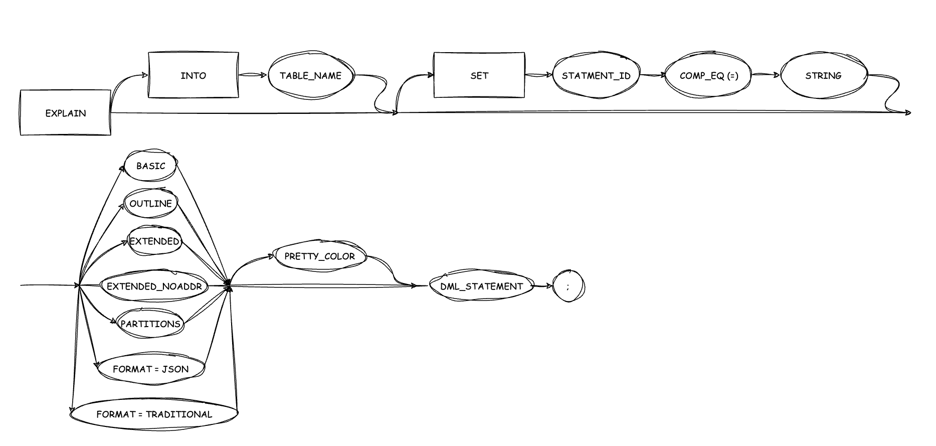
Syntax
{EXPLAIN [INTO table_name] [SET statement_id = string]}
[explain_type] [PRETTY | PRETTY_COLOR] dml_statement;

explain_type:
    BASIC
  | OUTLINE
  | EXTENDED
  | EXTENDED_NOADDR
  | PARTITIONS
  | FORMAT = {TRADITIONAL| JSON}

dml_statement:
    SELECT statement
  | DELETE statement
  | INSERT statement
  | REPLACE statement
Parameters
| Parameter | Description |
|---|---|
| INTO table_name | The table where the execution plan obtained by EXPLAIN is to be stored. If you do not specify INTO table_name, the execution plan is stored in the PLAN_TABLE table by default. |
| SET statement_id | The statement ID of the explained SQL statement, which can be used to query the execution plan of the statement later. If you do not specify SET statement_id, an empty string is used as the statement ID by default. |
| PRETTY | PRETTY_COLOR | Specifies to connect the parent and child nodes in the plan tree with tree lines or colored tree lines to make the execution plan easier to read. |
| BASIC | The basic information about the output plan, such as the operator ID, operator name, and name of the referenced table. |
| OUTLINE | The outline information contained in the output plan. |
| EXTENDED | Specifies to display the extra information. |
| EXTENDED_NOADDR | Specifies to display the brief extra information. |
| PARTITIONS | Specifies to display the partition-related information. |
FORMAT = {TRADITIONAL | JSON} | The output format of EXPLAIN. Valid values:
|
| dml_statement | The DML statement. |
The EXPLAIN and EXPLAIN EXTENDED_NOADDR statements are most commonly used in OceanBase Database.
-
The
EXPLAINstatement shows information that helps you understand the entire execution process of a plan. Here is an example:create table t1(c1 int, c2 int);
create table t2(c1 int, c2 int);
-- Insert 10 rows of test data into the `t1` table, and set values of the `c1` column to consecutive integers ranging from 1 to 1000.
insert into t1 with recursive cte(n) as (select 1 from dual union all select n + 1 from cte where n < 1000) select n, n from cte;
-- Insert 10 rows of test data into the `t2` table, and set values of the `c1` column to consecutive integers ranging from 1 to 1000.
insert into t2 with recursive cte(n) as (select 1 from dual union all select n + 1 from cte where n < 1000) select n, n from cte;
-- Collect statistics on the `t1` table.
analyze table t1 COMPUTE STATISTICS for all columns size 128;
-- Collect statistics on the `t2` table.
analyze table t2 COMPUTE STATISTICS for all columns size 128;
explain select * from t1, t2 where t1.c1 = t2.c1 and t1.c1 < 500;
+------------------------------------------------------------------------------------+
| Query Plan |
+------------------------------------------------------------------------------------+
| ================================================= |
| |ID|OPERATOR |NAME|EST.ROWS|EST.TIME(us)| |
| ------------------------------------------------- |
| |0 |HASH JOIN | |498 |315 | |
| |1 |├─TABLE FULL SCAN|t1 |499 |76 | |
| |2 |└─TABLE FULL SCAN|t2 |499 |76 | |
| ================================================= |
| Outputs & filters: |
| ------------------------------------- |
| 0 - output([t1.c1], [t1.c2], [t2.c1], [t2.c2]), filter(nil), rowset=256 |
| equal_conds([t1.c1 = t2.c1]), other_conds(nil) |
| 1 - output([t1.c1], [t1.c2]), filter([t1.c1 < 500]), rowset=256 |
| access([t1.c1], [t1.c2]), partitions(p0) |
| is_index_back=false, is_global_index=false, filter_before_indexback[false], |
| range_key([t1.__pk_increment]), range(MIN ; MAX)always true |
| 2 - output([t2.c1], [t2.c2]), filter([t2.c1 < 500]), rowset=256 |
| access([t2.c1], [t2.c2]), partitions(p0) |
| is_index_back=false, is_global_index=false, filter_before_indexback[false], |
| range_key([t2.__pk_increment]), range(MIN ; MAX)always true |
+------------------------------------------------------------------------------------+The following table describes columns of an execution plan in OceanBase Database.
Column Description ID The sequence number of the operator obtained by the execution tree through preorder traversal, starting from 0. OPERATOR The name of the operator. NAME The name of the table or index corresponding to a table operation. EST. ROWS The number of output rows of the operator estimated by the optimizer. This column is for your reference only.
In the preceding figure, Operator 1TABLE FULL SCANcontains the filter conditiont1.c1 < 500. Based on the statistics of the 1000 rows of data, the optimizer estimates that 499 rows of data are to be output.EST.TIME The execution cost of the operator estimated by the optimizer, in microseconds. This column is for your reference only. In a table operation, the
NAMEfield displays names (alias) of tables involved in the operation. In the case of index access, the name of the index is displayed in parentheses after the table name. For example,t1(t1_c2)indicates that indext1_c2is used. In the case of reverse scanning, the keywordRESERVEis added after the index name, with the index name and the keywordRESERVEseparated with a comma (,), such ast1(t1_c2,RESERVE).In OceanBase Database, the first part of the output of
EXPLAINis the tree structure of the execution plan. The hierarchy of operations in the tree is represented by the indentation of the operators. Operators at the deepest level are executed first. Operators at the same level are executed in the specified execution order. The following figure shows the tree structure of the execution plan described in the preceding example: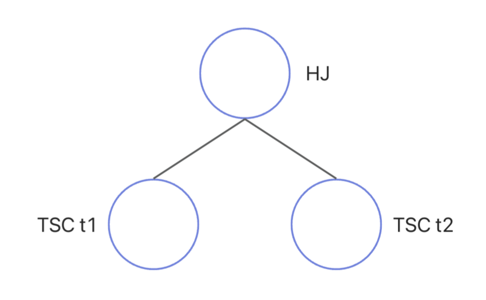
Operator 0 is a
HASH JOINoperator and has two subnodes: Operators 1 and 2, which areTABLE SCANoperators. The execution logic of Operator 0 is as follows:-
Read data from the subnode on the left to generate a hash value based on the join column, and then create a hash table.
-
Read data from the subnode on the right to generate a hash value based on the join column, and try to use the hash table created based on the data of the node on the left for hash probes to complete the join operation.
In OceanBase Database, the second part of the output of
EXPLAINcontains the details of each operator, including the output expression, filter conditions, partition information, and unique information of each operator, such as the sort keys, join keys, and pushdown conditions. The second part is the same as the second half of the preceding plan.Outputs & filters:
-------------------------------------
0 - output([t1.c1], [t1.c2], [t2.c1], [t2.c2]), filter(nil), rowset=16
equal_conds([t1.c1 = t2.c1]), other_conds(nil)
1 - output([t1.c1], [t1.c2]), filter([t1.c1 > 10]), rowset=16
access([t1.c1], [t1.c2]), partitions(p0)
is_index_back=false, is_global_index=false, filter_before_indexback[false],
range_key([t1.__pk_increment]), range(MIN ; MAX)always true
2 - output([t2.c1], [t2.c2]), filter([t2.c1 > 10]), rowset=16
access([t2.c1], [t2.c2]), partitions(p0)
is_index_back=false, is_global_index=false, filter_before_indexback[false],
range_key([t2.__pk_increment]), range(MIN ; MAX)always trueThe second part describes the details of operators in the first part. The common information includes:
-
output: The output expressions of the operator. -
filter: The filter predicates of the operator.filteris set tonilif no filter condition is configured for the operator.
To better understand each operator in the plan described in the second part of output of
EXPLAIN, you must first get familiar with the purposes of the operators. For more information, see Execution plan operators.For example, to understand the operators in the preceding plan, see TABLE SCAN and the HASH JOIN section in JOIN.
Note
rowset=16in the preceding plan is related to vectorized execution of the OceanBase Database execution engine. It specifies to calculate 16 rows of data at a time in a specific operator.You can specify
_rowsets_enabledto enable or disable vectorization. For example, thealter system set _rowsets_enabled = 0;statement disables vectorization. You can also specify_rowsets_max_rowsto set the number of rows to be processed at a time in vectorized execution. For example, thealter system set_rowsets_max_rows = 4;statement changes the number of rows to be processed at a time to4.For more information about vectorization, see the Vectorized execution section in Key Lightweight Data Warehouse Technologies of OceanBase Database.
-
-
The
EXPLAIN EXTENDED_NOADDRstatement extends a plan to its full frame with the most details and is usually used in troubleshooting.CREATE TABLE `t1` (
`c1` int, `c2` int,
KEY `idx` (`c1`));
insert into t1 values(1, 2);
explain EXTENDED_NOADDR select * from t1 where c1 > 10;
+--------------------------------------------------------------------------+
| Query Plan |
+--------------------------------------------------------------------------+
| =================================================== |
| |ID|OPERATOR |NAME |EST.ROWS|EST.TIME(us)| |
| --------------------------------------------------- |
| |0 |TABLE RANGE SCAN|t1(idx)|1 |7 | |
| =================================================== |
| Outputs & filters: |
| ------------------------------------- |
| 0 - output([t1.c1], [t1.c2]), filter(nil), rowset=16 |
| access([t1.__pk_increment], [t1.c1], [t1.c2]), partitions(p0) |
| is_index_back=true, is_global_index=false, |
| range_key([t1.c1], [t1.__pk_increment]), range(10,MAX ; MAX,MAX), |
| range_cond([t1.c1 > 10]) |
| Used Hint: |
| ------------------------------------- |
| /*+ |
| |
| */ |
| Qb name trace: |
| ------------------------------------- |
| stmt_id:0, stmt_type:T_EXPLAIN |
| stmt_id:1, SEL$1 |
| Outline Data: |
| ------------------------------------- |
| /*+ |
| BEGIN_OUTLINE_DATA |
| INDEX(@"SEL$1" "test"." t1"@"SEL$1" "idx") |
| OPTIMIZER_FEATURES_ENABLE('4.0.0.0') |
| END_OUTLINE_DATA |
| */ |
| Optimization Info: |
| ------------------------------------- |
| t1: |
| table_rows:1 |
| physical_range_rows:1 |
| logical_range_rows:1 |
| index_back_rows:1 |
| output_rows:1 |
| table_dop:1 |
| dop_method:Table DOP |
| avaiable_index_name: [idx, t1] |
| unstable_index_name: [t1] |
| stats version:0 |
| dynamic sampling level:0 |
| Plan Type: |
| LOCAL |
| Note: |
| Degree of Parallelisim is 1 because of table property |
+--------------------------------------------------------------------------+
47 rows in setThe information in the
Optimization Infosection helps you analyze performance issues of SQL statements. The following table describes the fields in theOptimization Infosection.Field Description table_rows The number of rows of the SSTable in the last major compaction version, which can be simply understood as the number of rows of the t1table. This field is for your reference only.physical_range_rows The number of physical rows of the t1table to be scanned. If an index is used, this field indicates the number of physical rows of thet1table to be scanned in the index.logical_range_rows The number of logical rows of the t1table to be scanned. If an index is used, this field indicates the number of logical rows of thet1table to be scanned in the index. In the preceding plan, the scan range isrange(10,MAX ; MAX,MAX),range_cond([t1.c1 > 10])because the indexidxis scanned. If no index is used, a full table scan is required. In this case, the scan range changes torange(MIN ; MAX).Notice
- Generally, the values of
physical_range_rowsandlogical_range_rowsare close. You can use either one. However, in special buffer tables, the value ofphysical_range_rowsmay be much larger than that oflogical_range_rows. - Data is frequently inserted to or deleted from buffer tables. If a large amount of incremental data is labeled as deleted in the LSM-tree architecture, few rows are actually available for upper-layer applications, and the labeled data may be processed during range queries. In this case, the value of
physical_range_rowsmay be much larger than that oflogical_range_rows, which results in long execution time of SQL queries. In the presence of buffer tables, the optimizer is prone to generate suboptimal execution plans. - For more information about the concept, detection logic, and troubleshooting methods for buffer tables, see Buffer tables.
index_back_rows The number of rows accessed by index primary key. The value 0indicates a full table scan or an index scan without table access by index primary key. For more information about table access by index primary key, see TABLE SCAN. Simply put, the primary table needs to be accessed by index primary key in the preceding plan because the indexidxcontains only the data of thec1column and the data of thec2column must be queried from the primary table based on the hidden primary keys of the primary table that correspond to the data filtered by the index. If theselect c1 from t1 where c1 > 10statement, rather than theselect * from t1 where c1 > 10statement, is executed, table access by index primary key is not required because the index contains all the information to be queried.output_rows The estimated number of output rows. In the preceding plan, this field indicates the number of rows of the t1table that are output after filtering.table_dop The degree of parallelism (DOP) for scanning the t1table. The DOP indicates the number of worker threads used for parallel execution.dop_method The method for determining the DOP for scanning the table. The value TableDOPindicates that the DOP is defined by the table. The valueAutoDopindicates that the DOP is selected by the optimizer based on the cost. In this case, the auto DOP feature must be enabled. The valueglobal parallelindicates that the DOP is specified by thePARALLELhint or a system variable.avaiable_index_name The list of indexes available for the t1table. The list contains index tables and the primary table. If no suitable index is available, the plan executes a full table scan on the primary table.pruned_index_name The list of indexes pruned by the current query based on the rules of the optimizer. For more information about the index pruning rules of the optimizer, see Rule-based path selection. unstable_index_name The pruned primary table path. The primary table path is usually pruned if an index path involving fewer rows is available. stats version The version of statistics about the t1table. The value0indicates that no statistics are collected for the table. To ensure correct generation of a plan, statistics about the table can be automatically or manually collected.dynamic sampling level The level of dynamic sampling. The value 0indicates that dynamic sampling is not enabled for the table.
Dynamic sampling is an optimization tool for the optimizer. For more information, see Dynamic sampling.estimation method The method for estimating the number of rows of the t1table. The valueDEFAULTindicates that the number of rows is estimated based on default statistics. In this case, the estimated number of rows can be inaccurate and must be optimized by the database administrator (DBA). The valueSTORAGEindicates that the number of rows is estimated in real time based on the storage layer. The valueSTATSindicates that the number of rows is estimated based on statistics.Plan Type The type of the current plan. Valid values: LOCAL,REMOTE, andDISTRIBUTED. For more information, see the Types of SQL execution plans section in '7.2 Principles of ODP SQL routing'Note The additional information for generating the plan. For example, in the preceding plan, Degree of Parallelisim is 1 because of table propertyindicates that the DOP of the current query is set to1because the DOP of the current table is set to1. - Generally, the values of
-
The
EXPLAIN EXTENDEDstatement further returns the data storage addresses of expressions involved in the operators in addition to the information returned by theEXPLAIN EXTENDED_NOADDRstatement. It is usually used by OceanBase Technical Support and R&D engineers in troubleshooting. The syntax is as follows:explain EXTENDED select * from t1 where c1 > 10;The output is as follows:
+---------------------------------------------------------------------------------------------------------------------+
| Query Plan                                                                                                          |
+---------------------------------------------------------------------------------------------------------------------+
| ===================================================                                                                 |
| |ID|OPERATOR        |NAME   |EST.ROWS|EST.TIME(us)|                                                                 |
| ---------------------------------------------------                                                                 |
| |0 |TABLE RANGE SCAN|t1(idx)|1       |7           |                                                                 |
| ===================================================                                                                 |
| Outputs & filters:                                                                                                  |
| -------------------------------------                                                                               |
|   0 - output([t1.c1(0x7fed4fe0df50)], [t1.c2(0x7fed4fe0e4c0)]), filter(nil), rowset=16                              |
|       access([t1.__pk_increment(0x7fed4fe0e9d0)], [t1.c1(0x7fed4fe0df50)], [t1.c2(0x7fed4fe0e4c0)]), partitions(p0) |
|       is_index_back=true, is_global_index=false,                                                                    |
|       range_key([t1.c1(0x7fed4fe0df50)], [t1.__pk_increment(0x7fed4fe0e9d0)]), range(10,MAX ; MAX,MAX),             |
|       range_cond([t1.c1(0x7fed4fe0df50) > 10(0x7fed4fe0d800)])                                                      |
|                                                                                                                     |
|       ......                                                                                                        |
|                                                                                                                     |
+---------------------------------------------------------------------------------------------------------------------+
Execution plan operators
For information about common operators, see Execution plan operators.
Note
We recommend that you get familiar with the TABLE SCAN and JOIN operators as well as DAS execution for the
TABLE SCANoperator.
This topic describes only the EXCHANGE operators. The EXCHANGE operators are commonly used in execution plans of OceanBase Database and not easy to understand. Therefore, this topic provides additional information based on related content in OceanBase Database documentation.
The EXCHANGE operators exchange data between threads and usually appear in pairs, with an EXCHANGE OUT operator on the source side and an EXCHANGE IN operator on the destination side. You can use the EXCHANGE operators to gather, transmit, and repartition data.
EXCHANGE IN/EXCHANGE OUT
The EXCHANGE IN and EXCHANGE OUT operators aggregate data from multiple partitions and send the aggregated data to the leader node involved in the query.
The following query accesses five partitions: p0, p1, p2, p3, and p4.
CREATE TABLE t3 (c1 INT, c2 INT) PARTITION BY HASH(c1) PARTITIONS 5;
Execute the EXPLAIN statement to query the execution plan.
explain select * from t3 where c1 > 10;
The output is as follows:
+------------------------------------------------------------------------------------+
| Query Plan                                                                         |
+------------------------------------------------------------------------------------+
| =============================================================                      |
| |ID|OPERATOR                 |NAME    |EST.ROWS|EST.TIME(us)|                      |
| -------------------------------------------------------------                      |
| |0 |PX COORDINATOR           |        |1       |20          |                      |
| |1 |└─EXCHANGE OUT DISTR     |:EX10000|1       |20          |                      |
| |2 |  └─PX PARTITION ITERATOR|        |1       |19          |                      |
| |3 |    └─TABLE FULL SCAN    |t3      |1       |19          |                      |
| =============================================================                      |
| Outputs & filters:                                                                 |
| -------------------------------------                                              |
|   0 - output([INTERNAL_FUNCTION(t3.c1, t3.c2)]), filter(nil), rowset=16            |
|   1 - output([INTERNAL_FUNCTION(t3.c1, t3.c2)]), filter(nil), rowset=16            |
|       dop=1                                                                        |
|   2 - output([t3.c1], [t3.c2]), filter(nil), rowset=16                             |
|       force partition granule                                                      |
|   3 - output([t3.c1], [t3.c2]), filter([t3.c1 > 10]), rowset=16                    |
|       access([t3.c1], [t3.c2]), partitions(p[0-4])                                 |
|       is_index_back=false, is_global_index=false, filter_before_indexback[false],  |
|       range_key([t3.__pk_increment]), range(MIN ; MAX)always true                  |
+------------------------------------------------------------------------------------+
The operators in the plan are described as follows:
-
Operator 2
PX PARTITION ITERATORiterates data by partition. For information about granule iterator (GI) operators, see GI. -
Operator 1
EXCHANGE OUT DISTRreceives the output of Operator 2PX PARTITION ITERATORand sends the data out. -
Operator 0
PX COORDINATORreceives the output of Operator 1 from multiple partitions, aggregates them, and returns the result.PX COORDINATORis a special type ofEXCHANGE INoperator, and is responsible for not only pulling back remote data, but also scheduling the execution of sub-plans.
EXCHANGE IN/EXCHANGE OUT (REMOTE)
OceanBase Database supports local, remote, and distributed plans. For more information, see '7.2 Principles of ODP SQL routing'. The EXCHANGE IN REMOTE and EXCHANGE OUT REMOTE operators are used in a remote plan to pull remote data in a single partition back to the local node.
Here is an example: A cluster is created in the 1-1-1 architecture, where the cluster has three zones and each zone has one node. The three zones are denoted as zone1, zone2, and zone3, and the three nodes are denoted as A, B, and C. primary_zone is set to zone1 for a tenant, and the leaders of all tables of the tenant are stored on node A in zone1.
Local plan
If you directly connect to node A to perform calculation for two non-partitioned tables, a local plan will be generated because the leaders of the two tables are stored on the local node. A sample plan is as follows:
create table t1(c1 int, c2 int);

create table t2(c1 int, c2 int);

explain select * from t1, t2 where t1.c1 = t2.c1 and t1.c1 > 10;
+------------------------------------------------------------------------------------+
| Query Plan                                                                         |
+------------------------------------------------------------------------------------+
| =================================================                                  |
| |ID|OPERATOR         |NAME|EST.ROWS|EST.TIME(us)|                                  |
| -------------------------------------------------                                  |
| |0 |HASH JOIN        |    |1       |9           |                                  |
| |1 |├─TABLE FULL SCAN|t1  |1       |4           |                                  |
| |2 |└─TABLE FULL SCAN|t2  |1       |4           |                                  |
| =================================================                                  |
| Outputs & filters: Omitted                                                              |
Remote plan
If you directly connect to node B to perform calculation for two non-partitioned tables, a remote plan will be generated because the leaders of the two tables are not stored on the local node. A sample plan is as follows:
explain select * from t1, t2 where t1.c1 = t2.c1 and t1.c1 > 10;
The output is as follows:
+------------------------------------------------------------------------------------+
| Query Plan                                                                         |
+------------------------------------------------------------------------------------+
| =====================================================                              |
| |ID|OPERATOR             |NAME|EST.ROWS|EST.TIME(us)|                              |
| -----------------------------------------------------                              |
| |0 |EXCHANGE IN REMOTE   |    |1       |11          |                              |
| |1 |└─EXCHANGE OUT REMOTE|    |1       |10          |                              |
| |2 |  └─HASH JOIN        |    |1       |9           |                              |
| |3 |    ├─TABLE FULL SCAN|t1  |1       |4           |                              |
| |4 |    └─TABLE FULL SCAN|t2  |1       |4           |                              |
| =====================================================                              |
| Outputs & filters:                                                                 |
| -------------------------------------                                              |
|   0 - output([t1.c1], [t1.c2], [t2.c1], [t2.c2]), filter(nil)                      |
|   1 - output([t1.c1], [t1.c2], [t2.c1], [t2.c2]), filter(nil)                      |
|   2 - output([t1.c1], [t1.c2], [t2.c1], [t2.c2]), filter(nil), rowset=16           |
|       equal_conds([t1.c1 = t2.c1]), other_conds(nil)                               |
|   3 - output([t1.c1], [t1.c2]), filter([t1.c1 > 10]), rowset=16                    |
|       access([t1.c1], [t1.c2]), partitions(p0)                                     |
|       is_index_back=false, is_global_index=false, filter_before_indexback[false],  |
|       range_key([t1.__pk_increment]), range(MIN ; MAX)always true                  |
|   4 - output([t2.c1], [t2.c2]), filter([t2.c1 > 10]), rowset=16                    |
|       access([t2.c1], [t2.c2]), partitions(p0)                                     |
|       is_index_back=false, is_global_index=false, filter_before_indexback[false],  |
|       range_key([t2.__pk_increment]), range(MIN ; MAX)always true                  |
+------------------------------------------------------------------------------------+
23 rows in set
The EXCHANGE IN REMOTE and EXCHANGE OUT REMOTE operators in the remote plan pull remote data in a single partition back to the local node.
In this case, Operators 0 and 1 are assigned to the execution plan to fetch remote data. The operators in the plan are described as follows:
-
Operators 2 to 4 are executed on node
Ato read data from the storage layer and complete theHASH JOINoperation. -
Operator 1
EXCHANGE OUT REMOTEis also executed on nodeAto read the result data calculated by Operator 2HASH JOINand send the data to Operator 0. -
Operator 0
EXCHANGE IN REMOTEis executed on nodeBto receive the output of Operator 1.
EXCHANGE IN/EXCHANGE OUT (PKEY)
The EXCHANGE IN/EXCHANGE OUT (PKEY) operators repartition data. They are generally used with a binary operator pair, such as a JOIN operator pair, to repartition the data of the left-side subnode by using the partitioning method of the right-side subnode and then send the repartitioned data to the OBServer node where the partition corresponding to the right-side subnode resides.
In the following example, the query joins two partitioned tables.
CREATE TABLE t1 (c1 INT, c2 INT) PARTITION BY HASH(c1) PARTITIONS 5;

CREATE TABLE t2 (c1 INT PRIMARY KEY, c2 INT) PARTITION BY HASH(c1) PARTITIONS 4;

EXPLAIN SELECT * FROM t1, t2 WHERE t1.c1 = t2.c1;
+---------------------------------------------------------------------------------------+
| Query Plan                                                                            |
+---------------------------------------------------------------------------------------+
| =====================================================================                 |
| |ID|OPERATOR                         |NAME    |EST.ROWS|EST.TIME(us)|                 |
| ---------------------------------------------------------------------                 |
| |0 |PX COORDINATOR                   |        |1       |38          |                 |
| |1 |└─EXCHANGE OUT DISTR             |:EX10001|1       |37          |                 |
| |2 |  └─HASH JOIN                    |        |1       |36          |                 |
| |3 |    ├─EXCHANGE IN DISTR          |        |1       |20          |                 |
| |4 |    │ └─EXCHANGE OUT DISTR (PKEY)|:EX10000|1       |20          |                 |
| |5 |    │   └─PX PARTITION ITERATOR  |        |1       |19          |                 |
| |6 |    │     └─TABLE FULL SCAN      |t1      |1       |19          |                 |
| |7 |    └─PX PARTITION ITERATOR      |        |1       |16          |                 |
| |8 |      └─TABLE FULL SCAN          |t2      |1       |16          |                 |
| =====================================================================                 |
| Outputs & filters:                                                                    |
| -------------------------------------                                                 |
|   0 - output([INTERNAL_FUNCTION(t1.c1, t1.c2, t2.c1, t2.c2)]), filter(nil), rowset=16 |
|   1 - output([INTERNAL_FUNCTION(t1.c1, t1.c2, t2.c1, t2.c2)]), filter(nil), rowset=16 |
|       dop=1                                                                           |
|   2 - output([t1.c1], [t2.c1], [t1.c2], [t2.c2]), filter(nil), rowset=16              |
|       equal_conds([t1.c1 = t2.c1]), other_conds(nil)                                  |
|   3 - output([t1.c1], [t1.c2]), filter(nil), rowset=16                                |
|   4 - output([t1.c1], [t1.c2]), filter(nil), rowset=16                                |
|       (#keys=1, [t1.c1]), dop=1                                                       |
|   5 - output([t1.c1], [t1.c2]), filter(nil), rowset=16                                |
|       force partition granule                                                         |
|   6 - output([t1.c1], [t1.c2]), filter(nil), rowset=16                                |
|       access([t1.c1], [t1.c2]), partitions(p[0-4])                                    |
|       is_index_back=false, is_global_index=false,                                     |
|       range_key([t1.__pk_increment]), range(MIN ; MAX)always true                     |
|   7 - output([t2.c1], [t2.c2]), filter(nil), rowset=16                                |
|       affinitize, force partition granule                                             |
|   8 - output([t2.c1], [t2.c2]), filter(nil), rowset=16                                |
|       access([t2.c1], [t2.c2]), partitions(p[0-3])                                    |
|       is_index_back=false, is_global_index=false,                                     |
|       range_key([t2.c1]), range(MIN ; MAX)always true                                 |
+---------------------------------------------------------------------------------------+
The execution plan repartitions the data of the t1 table by using the partitioning method of the t2 table.
-
Operator 4
EXCHANGE OUT DISTR (PKEY)determines the destination node for every row of thet1table based on the partitioning method of thet2table and the join condition of the query, and sends the rows of thet1table to corresponding nodes. -
Operator 3
EXCHANGE IN DISTRreceives the data of thet1table on corresponding nodes. -
Operator 2
HASH JOINexecutes aJOINoperation on each node to join the data iterated by Operator 7 and the data received by Operator 3. The data iterated by Operator 7 includes the data of all partitions of thet2table. The data received by Operator 3 includes the data of thet1table that is repartitioned based on the partitioning rules of thet2table. -
Operator 1
EXCHANGE OUT DISTRsends the join results to Operator 0. -
Operator 0
PX COORDINATORreceives and summarizes the join results from all nodes.
The optimizer also generates the EXCHANGE IN/EXCHANGE OUT (HASH) and EXCHANGE IN/EXCHANGE OUT (BC2HOST) operators based on different repartitioning methods for different SQL queries. For more information about repartitioning methods, see the Data distribution methods between the producer and the consumer section in Introduction to parallel execution.
Use hints to generate a plan
You can use hints to make the optimizer generate a specified execution plan. Generally, the optimizer will select the optimal execution plan for a query and you do not need to use a hint to specify an execution plan. However, in some scenarios, the execution plan generated by the optimizer may not meet your requirements. In this case, you need to use a hint to specify an execution plan to be generated.
Hint syntax
{ DELETE | INSERT | SELECT | UPDATE | REPLACE } /*+ [hint_text][,hint_text]... */
In the following query, the /*+ PARALLEL(3)*/ hint sets the DOP of SQL execution to 3. The EXPLAIN statement returns dop=3, and the explain EXTENDED_NOADDR statement additionally returns Note: Degree of Parallelism is 3 because of hint.
create t1 (c1 int, c2 int) PARTITION BY HASH(c1) PARTITIONS 5;

explain EXTENDED_NOADDR select /*+ PARALLEL(3) */* from t1 where c1 > 10;
+--------------------------------------------------------------------------+
| Query Plan                                                               |
+--------------------------------------------------------------------------+
| ==========================================================               |
| |ID|OPERATOR              |NAME    |EST.ROWS|EST.TIME(us)|               |
| ----------------------------------------------------------               |
| |0 |PX COORDINATOR        |        |1       |3           |               |
| |1 |└─EXCHANGE OUT DISTR  |:EX10000|1       |3           |               |
| |2 |  └─PX BLOCK ITERATOR |        |1       |3           |               |
| |3 |    └─TABLE RANGE SCAN|t1(idx) |1       |3           |               |
| ==========================================================               |
| Outputs & filters:                                                       |
| -------------------------------------                                    |
|   0 - output([INTERNAL_FUNCTION(t1.c1, t1.c2)]), filter(nil), rowset=16  |
|   1 - output([INTERNAL_FUNCTION(t1.c1, t1.c2)]), filter(nil), rowset=16  |
|       dop=3                                                              |
|   2 - output([t1.c1], [t1.c2]), filter(nil), rowset=16                   |
|   3 - output([t1.c1], [t1.c2]), filter(nil), rowset=16                   |
|       access([t1.__pk_increment], [t1.c1], [t1.c2]), partitions(p0)      |
|       is_index_back=true, is_global_index=false,                         |
|       range_key([t1.c1], [t1.__pk_increment]), range(10,MAX ; MAX,MAX),  |
|       range_cond([t1.c1 > 10])                                           |
| Used Hint:                                                               |
| -------------------------------------                                    |
|   /*+                                                                    |
|       PARALLEL(3)                                                        |
|   */                                                                     |
|                                                                          |
|   ......                                                                 |
|                                                                          |
|   Note:                                                                  |
|       Degree of Parallelism is 3 because of hint                         |
+--------------------------------------------------------------------------+
A hint is a special SQL comment in terms of syntax, because a plus sign (+) is added to the opening tag (/*) of the comment. If the OBServer node does not recognize the hint in an SQL statement due to syntax errors, the optimizer ignores the specified hint and generates a default execution plan. In addition, the hint only affects the execution plan generated by the optimizer. The semantics of the SQL statement remains unaffected.
Note
If you want to execute SQL statements containing hints in a MySQL client, you must log on to the client by using the
-coption. Otherwise, the MySQL client will remove the hints from the SQL statements as comments, and the system cannot receive the hints.
Hint parameters
The following table describes the name, syntax, and description of the hint parameters.
| Parameter | Syntax | Description |
|---|---|---|
| NO_REWRITE | NO_REWRITE | Specifies to prohibit SQL rewrite. |
| READ_CONSISTENCY | READ_CONSISTENCY(WEAK [STRONG]) | Sets the read consistency (weak/strong). |
| INDEX_HINT | INDEX(table_name index_name) | Sets the table index. |
| QUERY_TIMEOUT | QUERY_TIMEOUT(INTNUM) | Sets the statement timeout value. |
| LOG_LEVEL | LOG_LEVEL([']log_level[']) | Sets the log level. A module-level statement starts and ends with an apostrophe ('), for example, 'DEBUG'. |
| LEADING | LEADING([qb_name] TBL_NAME_LIST) | Sets the join order. |
| ORDERED | ORDERED | Specifies to join tables by the order in the SQL statement. |
| FULL | FULL([qb_name] TBL_NAME) | Specifies that the primary access path is equivalent to INDEX(TBL_NAME PRIMARY). |
| USE_PLAN_CACHE | USE_PLAN_CACHE(NONE[DEFAULT]) | Specifies whether to use the plan cache. Valid values:
|
| USE_MERGE | USE_MERGE([qb_name] TBL_NAME_LIST) | Specifies to use a merge join when the specified table is a right-side table. |
| USE_HASH | USE_HASH([qb_name] TBL_NAME_LIST) | Specifies to use a hash join when the specified table is a right-side table. |
| NO_USE_HASH | NO_USE_HASH([qb_name] TBL_NAME_LIST) | Specifies not to use a hash join when the specified table is a right-side table. |
| USE_NL | USE_NL([qb_name] TBL_NAME_LIST) | Specifies to use a nested loop join when the specified table is a right-side table. |
| USE_BNL | USE_BNL([qb_name] TBL_NAME_LIST) | Specifies to use a block nested loop join when the specified table is a right-side table. |
| USE_HASH_AGGREGATION | USE_HASH_AGGREGATION([qb_name]) | Sets the aggregation algorithm to a hash algorithm, such as HASH GROUP BY or HASH DISTINCT. |
| NO_USE_HASH_AGGREGATION | NO_USE_HASH_AGGREGATION([qb_name]) | Specifies to use MERGE GROUP BY or MERGE DISTINCT, rather than a hash aggregate algorithm, as the method to aggregate data. |
| USE_LATE_MATERIALIZATION | USE_LATE_MATERIALIZATION | Specifies to use LATE MATERIALIZATION. |
| NO_USE_LATE_MATERIALIZATION | NO_USE_LATE_MATERIALIZATION | Specifies not to use LATE MATERIALIZATION. |
| TRACE_LOG | TRACE_LOG | Specifies to collect the trace log for SHOW TRACE. |
| QB_NAME | QB_NAME( NAME ) | Sets the name of the query block. |
| PARALLEL | PARALLEL(INTNUM) | Sets the degree of parallelism (DOP) for distributed execution. |
| TOPK | TOPK(PRECISION MINIMUM_ROWS) | Specifies the precision and the minimum number of rows of a fuzzy query. The value of PRECISION is an integer within the range of [0, 100], which means the percentage of rows queried in a fuzzy query. MINIMUM_ROWS specifies the minimum number of returned rows. |
| MAX_CONCURRENT | MAX_CONCURRENT(n) | Specifies the maximum DOP for the SQL statement. |
Note
The syntax of
QB_NAMEis@NAME.The syntax of
TBL_NAMEis[db_name.]relation_name [qb_name].
QB_NAME
In DML statements, each query block has a query block name indicated by QB_NAME, which can be specified or automatically generated by the system. Each query block is a semantically complete query statement. Simply put, SELECT, DELETE, and similar keywords are extracted from SQL statements, structured, and then identified from left to right.
If you do not use a hint to specify QB_NAME, the system generates the names such as SEL$1, SEL$2, UPD$1, and DEL$1 from left to right, which is the operation order of the resolver.
You can use QB_NAME to accurately locate every table and specify the behavior of any query block at one position. QB_NAME in TBL_NAME is used to locate the table, and the first query block name in the hint is used to locate the query block to which the hint applies.
For example, the following rules apply to the SELECT *FROM t1, (SELECT* FROM t2 WHERE c2 = 1 LIMIT 5) WHERE t1.c1 = 1; statement by default:
-
The first query block
SEL$1is the outermost statement:SELECT * FROM t1, VIEW1 WHERE t1.c1 = 1. -
The second query block
SEL$2isANONYMOUS_VIEW1in the plan:SELECT * FROM t2 WHERE c2 = 1 LIMIT 5.
The optimizer selects the index t1_c1 for the t1 table in SEL$1 and primary table access for the t2 table in SEL$2.
CREATE TABLE t1(c1 INT, c2 INT, KEY t1_c1(c1));

CREATE TABLE t2(c1 INT, c2 INT, KEY t2_c1(c1));

EXPLAIN EXTENDED_NOADDR SELECT * FROM t1, (SELECT * FROM t2 WHERE c2 = 1 LIMIT 5) WHERE t1.c1 = 1;
+-----------------------------------------------------------------------------------------------------------+
| Query Plan                                                                                                |
+-----------------------------------------------------------------------------------------------------------+
| ======================================================================                                    |
| |ID|OPERATOR                   |NAME           |EST.ROWS|EST.TIME(us)|                                    |
| ----------------------------------------------------------------------                                    |
| |0 |NESTED-LOOP JOIN CARTESIAN |               |1       |11          |                                    |
| |1 |├─TABLE RANGE SCAN         |t1(t1_c1)      |1       |7           |                                    |
| |2 |└─MATERIAL                 |               |1       |4           |                                    |
| |3 |  └─SUBPLAN SCAN           |ANONYMOUS_VIEW1|1       |4           |                                    |
| |4 |    └─TABLE FULL SCAN      |t2             |1       |4           |                                    |
| ======================================================================                                    |
| Outputs & filters:                                                                                        |
| -------------------------------------                                                                     |
|   0 - output([t1.c1], [t1.c2], [.c1], [.c2]), filter(nil), rowset=16                                      |
|       conds(nil), nl_params_(nil), use_batch=false                                                        |
|   1 - output([t1.c1], [t1.c2]), filter(nil), rowset=16                                                    |
|       access([t1.__pk_increment], [t1.c1], [t1.c2]), partitions(p0)                                       |
|       is_index_back=true, is_global_index=false,                                                          |
|       range_key([t1.c1], [t1.__pk_increment]), range(1,MIN ; 1,MAX),                                      |
|       range_cond([t1.c1 = 1])                                                                             |
|   2 - output([.c1], [.c2]), filter(nil), rowset=16                                                        |
|   3 - output([.c1], [.c2]), filter(nil), rowset=16                                                        |
|       access([.c1], [.c2])                                                                                |
|   4 - output([t2.c1], [t2.c2]), filter([t2.c2 = 1]), rowset=16                                            |
|       access([t2.c2], [t2.c1]), partitions(p0)                                                            |
|       limit(5), offset(nil), is_index_back=false, is_global_index=false, filter_before_indexback[false],  |
|       range_key([t2.__pk_increment]), range(MIN ; MAX)always true                                         |
| Used Hint:                                                                                                |
| -------------------------------------                                                                     |
|   /*+                                                                                                     |
|                                                                                                           |
|   */                                                                                                      |
| Qb name trace:                                                                                            |
| -------------------------------------                                                                     |
|   stmt_id:0, stmt_type:T_EXPLAIN                                                                          |
|   stmt_id:1, SEL$1                                                                                        |
|   stmt_id:2, SEL$2                                                                                        |
| Outline Data:                                                                                             |
| -------------------------------------                                                                     |
|   /*+                                                                                                     |
|       BEGIN_OUTLINE_DATA                                                                                  |
|       LEADING(@"SEL$1" ("test"." t1"@"SEL$1" "ANONYMOUS_VIEW1"@"SEL$1"))                                   |
|       USE_NL(@"SEL$1" "ANONYMOUS_VIEW1"@"SEL$1")                                                          |
|       USE_NL_MATERIALIZATION(@"SEL$1" "ANONYMOUS_VIEW1"@"SEL$1")                                          |
|       INDEX(@"SEL$1" "test"." t1"@"SEL$1" "t1_c1")                                                         |
|       FULL(@"SEL$2" "test"." t2"@"SEL$2")                                                                  |
|       OPTIMIZER_FEATURES_ENABLE('4.0.0.0')                                                                |
|       END_OUTLINE_DATA                                                                                    |
|   */                                                                                                      |
|   ......                                                                                                  |
+-----------------------------------------------------------------------------------------------------------+
The following example uses a hint in an SQL statement to specify the access method of the t1 table in SEL$1 to primary table access, and that of the t2 table in SEL$2 to index access.
EXPLAIN EXTENDED_NOADDR
SELECT /*+ INDEX(@SEL$1 t1 PRIMARY) INDEX(@SEL$2 t2 t2_c1) */ *
FROM t1 , (SELECT * FROM t2 WHERE c2 = 1 LIMIT 5) WHERE t1.c1 = 1;
+----------------------------------------------------------------------------------------------------------+
| Query Plan                                                                                               |
+----------------------------------------------------------------------------------------------------------+
| ======================================================================                                   |
| |ID|OPERATOR                   |NAME           |EST.ROWS|EST.TIME(us)|                                   |
| ----------------------------------------------------------------------                                   |
| |0 |NESTED-LOOP JOIN CARTESIAN |               |1       |11          |                                   |
| |1 |├─TABLE FULL SCAN          |t1             |1       |4           |                                   |
| |2 |└─MATERIAL                 |               |1       |7           |                                   |
| |3 |  └─SUBPLAN SCAN           |ANONYMOUS_VIEW1|1       |7           |                                   |
| |4 |    └─TABLE FULL SCAN      |t2(t2_c1)      |1       |7           |                                   |
| ======================================================================                                   |
| Outputs & filters:                                                                                       |
| -------------------------------------                                                                    |
|   0 - output([t1.c1], [t1.c2], [.c1], [.c2]), filter(nil), rowset=16                                     |
|       conds(nil), nl_params_(nil), use_batch=false                                                       |
|   1 - output([t1.c1], [t1.c2]), filter([t1.c1 = 1]), rowset=16                                           |
|       access([t1.c1], [t1.c2]), partitions(p0)                                                           |
|       is_index_back=false, is_global_index=false, filter_before_indexback[false],                        |
|       range_key([t1.__pk_increment]), range(MIN ; MAX)always true                                        |
|   2 - output([.c1], [.c2]), filter(nil), rowset=16                                                       |
|   3 - output([.c1], [.c2]), filter(nil), rowset=16                                                       |
|       access([.c1], [.c2])                                                                               |
|   4 - output([t2.c1], [t2.c2]), filter([t2.c2 = 1]), rowset=16                                           |
|       access([t2.__pk_increment], [t2.c2], [t2.c1]), partitions(p0)                                      |
|       limit(5), offset(nil), is_index_back=true, is_global_index=false, filter_before_indexback[false],  |
|       range_key([t2.c1], [t2.__pk_increment]), range(MIN,MIN ; MAX,MAX)always true                       |
| Used Hint:                                                                                               |
| -------------------------------------                                                                    |
|   /*+                                                                                                    |
|                                                                                                          |
|       INDEX("t1" "primary")                                                                              |
|       INDEX(@"SEL$2" "t2" "t2_c1")                                                                       |
|   */                                                                                                     |
| Qb name trace:                                                                                           |
| -------------------------------------                                                                    |
|   stmt_id:0, stmt_type:T_EXPLAIN                                                                         |
|   stmt_id:1, SEL$1                                                                                       |
|   stmt_id:2, SEL$2                                                                                       |
| Outline Data:                                                                                            |
| -------------------------------------                                                                    |
|   /*+                                                                                                    |
|       BEGIN_OUTLINE_DATA                                                                                 |
|       LEADING(@"SEL$1" ("test"." t1"@"SEL$1" "ANONYMOUS_VIEW1"@"SEL$1"))                                  |
|       USE_NL(@"SEL$1" "ANONYMOUS_VIEW1"@"SEL$1")                                                         |
|       USE_NL_MATERIALIZATION(@"SEL$1" "ANONYMOUS_VIEW1"@"SEL$1")                                         |
|       FULL(@"SEL$1" "test"." t1"@"SEL$1")                                                                 |
|       INDEX(@"SEL$2" "test"." t2"@"SEL$2" "t2_c1")                                                        |
|       OPTIMIZER_FEATURES_ENABLE('4.0.0.0')                                                               |
|       END_OUTLINE_DATA                                                                                   |
|   */                                                                                                     |
|   ......                                                                                                 |
+----------------------------------------------------------------------------------------------------------+
You can observe the changes in the Query Plan and Outline Data sections after the hint /*+ INDEX(t1 PRIMARY) INDEX(@SEL$2 t2 t2_c1)*/ is specified and determine whether the changes are expected.
You can also rewrite the preceding hint in the following three ways, which are equivalent:
-
Method 1:
SELECT /*+INDEX(@SEL$1 t1 PRIMARY) INDEX(@SEL$2 t2 t2_c1)*/ * FROM t1 , (SELECT * FROM t2 WHERE c2 = 1 LIMIT 5) WHERE t1.c1 = 1; -
Method 2:
SELECT /*+INDEX(t1 PRIMARY) INDEX(@SEL$2 t2@SEL$2 t2_c1)*/ * FROM t1 , (SELECT * FROM t2 WHERE c2 = 1 LIMIT 5) WHERE t1.c1 = 1; -
Method 3:
SELECT /*+INDEX(t1 PRIMARY)*/ * FROM t1 , (SELECT /*+INDEX(t2 t2_c1)*/ * FROM t2 WHERE c2 = 1 LIMIT 5) WHERE t1.c1 = 1;
Usage rules of hints
Observe the following rules when you use hints:
-
A hint applies to the query block where it resides, if no query block is specified.
-
Example 1: The hint cannot take effect because it is written in query block 1 but the
t2table resides in query block 2 and the optimizer cannot relocate thet2table inSEL$2toSEL$1by rewriting the SQL statement.EXPLAIN SELECT /*+INDEX(t2 t2_c1)*/ *
FROM t1 , (SELECT * FROM t2 WHERE c2 = 1 LIMIT 5)
WHERE t1.c1 = 1;The output is as follows:
+-----------------------------------------------------------------------------------------------------------+
| Query Plan                                                                                                |
+-----------------------------------------------------------------------------------------------------------+
| ======================================================================                                    |
| |ID|OPERATOR                   |NAME           |EST.ROWS|EST.TIME(us)|                                    |
| ----------------------------------------------------------------------                                    |
| |0 |NESTED-LOOP JOIN CARTESIAN |               |1       |11          |                                    |
| |1 |├─TABLE RANGE SCAN         |t1(t1_c1)      |1       |7           |                                    |
| |2 |└─MATERIAL                 |               |1       |4           |                                    |
| |3 |  └─SUBPLAN SCAN           |ANONYMOUS_VIEW1|1       |4           |                                    |
| |4 |    └─TABLE FULL SCAN      |t2             |1       |4           |                                    |
| ======================================================================                                    |
| ......                                                                                                    |
+-----------------------------------------------------------------------------------------------------------+ -
Example 2: The hint takes effect because the optimizer can relocate the
t2table toSEL$1by rewriting the SQL statement. In the following plan, the original SQL statement is rewritten into one without an anonymous view:SELECT /*+INDEX(t2 t2_c1)*/ * FROM t1, t2 WHERE t1.c1 = 1 and t2.c2 = 1;. In the rewritten SQL statement, the hint takes effect because thet2table is relocated to the outermost query blockSEL$1.EXPLAIN SELECT /*+ INDEX(t2 t2_c1) */ *
FROM t1 , (SELECT * FROM t2 WHERE c2 = 1)
WHERE t1.c1 = 1;The output is as follows:
+------------------------------------------------------------------------------------+
| Query Plan                                                                         |
+------------------------------------------------------------------------------------+
| ================================================================                   |
| |ID|OPERATOR                   |NAME     |EST.ROWS|EST.TIME(us)|                   |
| ----------------------------------------------------------------                   |
| |0 |NESTED-LOOP JOIN CARTESIAN |         |1       |13          |                   |
| |1 |├─TABLE RANGE SCAN         |t1(t1_c1)|1       |7           |                   |
| |2 |└─MATERIAL                 |         |1       |7           |                   |
| |3 |  └─TABLE FULL SCAN        |t2(t2_c1)|1       |7           |                   |
| ================================================================                   |
| Outputs & filters:                                                                 |
| -------------------------------------                                              |
|   0 - output([t1.c1], [t1.c2], [t2.c1], [t2.c2]), filter(nil), rowset=16           |
|       conds(nil), nl_params_(nil), use_batch=false                                 |
|   1 - output([t1.c1], [t1.c2]), filter(nil), rowset=16                             |
|       access([t1.__pk_increment], [t1.c1], [t1.c2]), partitions(p0)                |
|       is_index_back=true, is_global_index=false,                                   |
|       range_key([t1.c1], [t1.__pk_increment]), range(1,MIN ; 1,MAX),               |
|       range_cond([t1.c1 = 1])                                                      |
|   2 - output([t2.c1], [t2.c2]), filter(nil), rowset=16                             |
|   3 - output([t2.c2], [t2.c1]), filter([t2.c2 = 1]), rowset=16                     |
|       access([t2.__pk_increment], [t2.c2], [t2.c1]), partitions(p0)                |
|       is_index_back=true, is_global_index=false, filter_before_indexback[false],   |
|       range_key([t2.c1], [t2.__pk_increment]), range(MIN,MIN ; MAX,MAX)always true |
+------------------------------------------------------------------------------------+
-
-
If a table is specified but is not found in the query block where the hint resides, or a conflict occurs, the hint is invalid.
Common hints
Compared with the optimizer behaviors of other databases, the behaviors of the OceanBase Database optimizer are dynamically planned, and all possible optimal paths have been considered. Hints are mainly used to specify the behavior of the optimizer, and SQL queries are executed based on the hints. This section describes the most commonly used hints.
INDEX hint
The syntax of the INDEX hint is as follows:
SELECT/*+ INDEX(table_name index_name) */ * FROM table_name;
If the SQL syntax contains table_name [AS] alias, you must specify a table alias for an INDEX hint to take effect. Here is an example:
create table t1(c1 int, c2 int, c3 int);

create index idx1 on t1(c1);

create index idx2 on t1(c2);

-- Insert 1000 rows of test data.
insert into t1 with recursive cte(n) as (select 1 from dual union all select n + 1 from cte where n < 1000) select n, mod(n, 3), n from cte;

-- Collect statistics on the `t1` table.
analyze table t1 COMPUTE STATISTICS for all columns size 128;

-- `c1 = 1` achieves better filtering effect for the 1000 rows of test data than `c2 = 1`.
-- Therefore, the optimizer preferentially selects the index `idx1` for generating a plan when the `INDEX` hint is not specified or does not take effect.
explain select * from t1 where c1 = 1 and c2 = 1;
+-----------------------------------------------------------------------------------+
| Query Plan                                                                        |
+-----------------------------------------------------------------------------------+
| ====================================================                              |
| |ID|OPERATOR        |NAME    |EST.ROWS|EST.TIME(us)|                              |
| ----------------------------------------------------                              |
| |0 |TABLE RANGE SCAN|t1(idx1)|1       |7           |                              |
| ====================================================                              |
| Outputs & filters:                                                                |
| -------------------------------------                                             |
|   0 - output([t1.c1], [t1.c2], [t1.c3]), filter([t1.c2 = 1]), rowset=16           |
|       access([t1.__pk_increment], [t1.c1], [t1.c2], [t1.c3]), partitions(p0)      |
|       is_index_back=true, is_global_index=false, filter_before_indexback[false],  |
|       range_key([t1.c1], [t1.__pk_increment]), range(1,MIN ; 1,MAX),              |
|       range_cond([t1.c1 = 1])                                                     |
+-----------------------------------------------------------------------------------+

-- The `INDEX` hint takes effect.
explain select /*+index(t idx2)*/ * from t1 as t where c1 = 1 and c2 = 1;
+-----------------------------------------------------------------------------------+
| Query Plan                                                                        |
+-----------------------------------------------------------------------------------+
| ===================================================                               |
| |ID|OPERATOR        |NAME   |EST.ROWS|EST.TIME(us)|                               |
| ---------------------------------------------------                               |
| |0 |TABLE RANGE SCAN|t(idx2)|1       |871         |                               |
| ===================================================                               |
| Outputs & filters:                                                                |
| -------------------------------------                                             |
|   0 - output([t.c1], [t.c2], [t.c3]), filter([t.c1 = 1]), rowset=16               |
|       access([t. __pk_increment], [t.c1], [t.c2], [t.c3]), partitions(p0)          |
|       is_index_back=true, is_global_index=false, filter_before_indexback[false],  |
|       range_key([t.c2], [t. __pk_increment]), range(1,MIN ; 1,MAX),                |
|       range_cond([t.c2 = 1])                                                      |
+-----------------------------------------------------------------------------------+

-- The `INDEX` hint does not take effect because the `t1` table is assigned the alias `t`.
explain select /*+index(t1 idx2)*/ * from t1 t where c1 = 1 and c2 = 1;
+-----------------------------------------------------------------------------------+
| Query Plan                                                                        |
+-----------------------------------------------------------------------------------+
| ===================================================                               |
| |ID|OPERATOR        |NAME   |EST.ROWS|EST.TIME(us)|                               |
| ---------------------------------------------------                               |
| |0 |TABLE RANGE SCAN|t(idx1)|1       |7           |                               |
| ===================================================                               |
| Outputs & filters:                                                                |
| -------------------------------------                                             |
|   0 - output([t.c1], [t.c2], [t.c3]), filter([t.c2 = 1]), rowset=16               |
|       access([t. __pk_increment], [t.c1], [t.c2], [t.c3]), partitions(p0)          |
|       is_index_back=true, is_global_index=false, filter_before_indexback[false],  |
|       range_key([t.c1], [t. __pk_increment]), range(1,MIN ; 1,MAX),                |
|       range_cond([t.c1 = 1])                                                      |
+-----------------------------------------------------------------------------------+
FULL hint
The syntax of the FULL hint specifies to scan the primary table. It is equivalent to the INDEX hint /*+ INDEX(table_name PRIMARY)*/.
Here is an example:
create table t1(c1 int, c2 int, c3 int);

create index idx1 on t1(c1);

-- The `c1` column has an index `idx1`, and both the column in the filter condition and the result column are `c1`. Therefore, the optimizer selects `idx1` by default.
explain select c1 from t1 where c1 = 1;
+-----------------------------------------------------------------------+
| Query Plan                                                            |
+-----------------------------------------------------------------------+
| ====================================================                  |
| |ID|OPERATOR        |NAME    |EST.ROWS|EST.TIME(us)|                  |
| ----------------------------------------------------                  |
| |0 |TABLE RANGE SCAN|t1(idx1)|1       |4           |                  |
| ====================================================                  |
| Outputs & filters:                                                    |
| -------------------------------------                                 |
|   0 - output([t1.c1]), filter(nil), rowset=4                          |
|       access([t1.c1]), partitions(p0)                                 |
|       is_index_back=false, is_global_index=false,                     |
|       range_key([t1.c1], [t1.__pk_increment]), range(1,MIN ; 1,MAX),  |
|       range_cond([t1.c1 = 1])                                         |
+-----------------------------------------------------------------------+

-- Use a hint to specify a full table scan.
explain select /*+ FULL(t1) */ c1 from t1 where c1 = 1;
+------------------------------------------------------------------------------------+
| Query Plan                                                                         |
+------------------------------------------------------------------------------------+
| ===============================================                                    |
| |ID|OPERATOR       |NAME|EST.ROWS|EST.TIME(us)|                                    |
| -----------------------------------------------                                    |
| |0 |TABLE FULL SCAN|t1  |1       |4           |                                    |
| ===============================================                                    |
| Outputs & filters:                                                                 |
| -------------------------------------                                              |
|   0 - output([t1.c1]), filter([t1.c1 = 1]), rowset=4                               |
|       access([t1.c1]), partitions(p0)                                              |
|       is_index_back=false, is_global_index=false, filter_before_indexback[false],  |
|       range_key([t1.__pk_increment]), range(MIN ; MAX)always true                  |
+------------------------------------------------------------------------------------+

-- Use a hint to specify a full table scan. The following statement is equivalent to the preceding one.
explain select /*+ index(t1 PRIMARY) */ c1 from t1 where c1 = 1;
+------------------------------------------------------------------------------------+
| Query Plan                                                                         |
+------------------------------------------------------------------------------------+
| ===============================================                                    |
| |ID|OPERATOR       |NAME|EST.ROWS|EST.TIME(us)|                                    |
| -----------------------------------------------                                    |
| |0 |TABLE FULL SCAN|t1  |1       |4           |                                    |
| ===============================================                                    |
| Outputs & filters:                                                                 |
| -------------------------------------                                              |
|   0 - output([t1.c1]), filter([t1.c1 = 1]), rowset=4                               |
|       access([t1.c1]), partitions(p0)                                              |
|       is_index_back=false, is_global_index=false, filter_before_indexback[false],  |
|       range_key([t1.__pk_increment]), range(MIN ; MAX)always true                  |
+------------------------------------------------------------------------------------+
LEADING hint
The LEADING hint specifies the order in which tables are joined. The syntax is as follows: /*+ LEADING(table_name_list)*/. You can use () in table_name_list to indicate the join priorities of right-side tables to specify a complex join. It is more flexible than the ORDERED hint. Here is an example:
EXPLAIN BASIC SELECT /*+LEADING(d c b a)*/ * FROM t1 a, t1 b, t1 c, t1 d;
+------------------------------------------------------------------------------------------------------+
| Query Plan                                                                                           |
+------------------------------------------------------------------------------------------------------+
| =========================================                                                            |
| |ID|OPERATOR                       |NAME|                                                            |
| -----------------------------------------                                                            |
| |0 |NESTED-LOOP JOIN CARTESIAN     |    |                                                            |
| |1 |├─NESTED-LOOP JOIN CARTESIAN   |    |                                                            |
| |2 |│ ├─NESTED-LOOP JOIN CARTESIAN |    |                                                            |
| |3 |│ │ ├─TABLE FULL SCAN          |d   |                                                            |
| |4 |│ │ └─MATERIAL                 |    |                                                            |
| |5 |│ │   └─TABLE FULL SCAN        |c   |                                                            |
| |6 |│ └─MATERIAL                   |    |                                                            |
| |7 |│   └─TABLE FULL SCAN          |b   |                                                            |
| |8 |└─MATERIAL                     |    |                                                            |
| |9 |  └─TABLE FULL SCAN            |a   |                                                            |
| =========================================                                                            |
+------------------------------------------------------------------------------------------------------+

EXPLAIN BASIC SELECT /*+LEADING((d c) (b a))*/ * FROM  t1 a, t1 b, t1 c, t1 d;
+------------------------------------------------------------------------------------------------------+
| Query Plan                                                                                           |
+------------------------------------------------------------------------------------------------------+
| =========================================                                                            |
| |ID|OPERATOR                       |NAME|                                                            |
| -----------------------------------------                                                            |
| |0 |NESTED-LOOP JOIN CARTESIAN     |    |                                                            |
| |1 |├─NESTED-LOOP JOIN CARTESIAN   |    |                                                            |
| |2 |│ ├─TABLE FULL SCAN            |d   |                                                            |
| |3 |│ └─MATERIAL                   |    |                                                            |
| |4 |│   └─TABLE FULL SCAN          |c   |                                                            |
| |5 |└─MATERIAL                     |    |                                                            |
| |6 |  └─NESTED-LOOP JOIN CARTESIAN |    |                                                            |
| |7 |    ├─TABLE FULL SCAN          |b   |                                                            |
| |8 |    └─MATERIAL                 |    |                                                            |
| |9 |      └─TABLE FULL SCAN        |a   |                                                            |
| =========================================                                                            |
+------------------------------------------------------------------------------------------------------+

EXPLAIN BASIC SELECT /*+LEADING((d c b) a))*/ * FROM t1 a, t1 b, t1 c, t1 d;
+------------------------------------------------------------------------------------------------------+
| Query Plan                                                                                           |
+------------------------------------------------------------------------------------------------------+
| =========================================                                                            |
| |ID|OPERATOR                       |NAME|                                                            |
| -----------------------------------------                                                            |
| |0 |NESTED-LOOP JOIN CARTESIAN     |    |                                                            |
| |1 |├─NESTED-LOOP JOIN CARTESIAN   |    |                                                            |
| |2 |│ ├─NESTED-LOOP JOIN CARTESIAN |    |                                                            |
| |3 |│ │ ├─TABLE FULL SCAN          |d   |                                                            |
| |4 |│ │ └─MATERIAL                 |    |                                                            |
| |5 |│ │   └─TABLE FULL SCAN        |c   |                                                            |
| |6 |│ └─MATERIAL                   |    |                                                            |
| |7 |│   └─TABLE FULL SCAN          |b   |                                                            |
| |8 |└─MATERIAL                     |    |                                                            |
| |9 |  └─TABLE FULL SCAN            |a   |                                                            |
| =========================================                                                            |
+------------------------------------------------------------------------------------------------------+
The LEADING hint is strictly examined to ensure that tables are joined in the order specified by the user. The LEADING hint becomes invalid if table_name specified in the hint does not exist, or duplicate tables are found in the hint. If the optimizer does not find a table in FROM items by table_id during a JOIN operation, the query may have been rewritten. In this case, the join order for this table and tables after this table is invalid. The join order before the table is still valid.
Note
When
ORDEREDandLEADINGhints are used at the same time, only theORDEREDhint takes effect.
USE_NL hint
The syntax of a hint that uses a join algorithm is join_hint_name ( @ qb_name table_name_list). When the right-side table in the join matches table_name_list, the optimizer generates a plan based on the hint semantics. Generally, you need to use a LEADING hint to specify the join order to make sure that the table in table_name_list is the right-side table. Otherwise, the hint becomes invalid as the join order changes.
table_name_list supports the following forms:
-
USE_NL(t1): uses the nested loop join algorithm when thet1table is the right-side table. -
USE_NL(t1 t2 ... ): uses the nested loop join algorithm when thet1ort2table or any other one in the list is the right-side table. -
USE_NL((t1 t2)): uses the nested loop join algorithm when the join result of thet1andt2tables is the right-side table. The join order and method of thet1andt2tables are ignored. -
USE_NL(t1 (t2 t3) (t4 t5 t6) ... ): uses the nested loop join algorithm when thet1table, the join result of thet2andt3tables, the join result of thet4,t5, andt6tables, or any other item in the list is the right-side table.
The USE_NL hint specifies to use the nested loop join algorithm for a join when the specified table is a right-side table. The syntax is as follows: /*+ USE_NL(table_name_list)*/. Here is an example:
CREATE TABLE t0(c1 INT, c2 INT, c3 INT);

CREATE TABLE t1(c1 INT, c2 INT, c3 INT);

CREATE TABLE t2(c1 INT, c2 INT, c3 INT);

-- If you want to join the `t0` table with the `t1` table in a nested loop join, specify the hint as follows:
EXPLAIN BASIC SELECT /*+ LEADING(t0 t1) USE_NL(t1) */ * FROM t0, t1 WHERE t0.c1 = t1.c1;
+--------------------------------------------------------------------------------------------+
| Query Plan                                                                                 |
+--------------------------------------------------------------------------------------------+
| =============================                                                              |
| |ID|OPERATOR           |NAME|                                                              |
| -----------------------------                                                              |
| |0 |NESTED-LOOP JOIN   |    |                                                              |
| |1 |├─TABLE FULL SCAN  |t0  |                                                              |
| |2 |└─MATERIAL         |    |                                                              |
| |3 |  └─TABLE FULL SCAN|t1  |                                                              |
| =============================                                                              |
+--------------------------------------------------------------------------------------------+

-- If you want to join the `t0` table with the join result of the `t1` and `t2` tables with the outermost join as a nested loop join, specify the hint as follows:
EXPLAIN BASIC SELECT /*+ LEADING(t0 (t1 t2)) USE_NL((t1 t2)) */ * FROM t0, t1, t2 WHERE t0.c1 = t1.c1 AND t0.c1 = t2.c1;
+-----------------------------------------------------------------------------------------------------------------------+
| Query Plan                                                                                                            |
+-----------------------------------------------------------------------------------------------------------------------+
| ===============================                                                                                       |
| |ID|OPERATOR             |NAME|                                                                                       |
| -------------------------------                                                                                       |
| |0 |NESTED-LOOP JOIN     |    |                                                                                       |
| |1 |├─TABLE FULL SCAN    |t0  |                                                                                       |
| |2 |└─MATERIAL           |    |                                                                                       |
| |3 |  └─HASH JOIN        |    |                                                                                       |
| |4 |    ├─TABLE FULL SCAN|t1  |                                                                                       |
| |5 |    └─TABLE FULL SCAN|t2  |                                                                                       |
| ===============================                                                                                       |
+-----------------------------------------------------------------------------------------------------------------------+
Notice
The
USE_NL,USE_HASH, andUSE_MERGEhints are usually used with theLEADINGhint because the optimizer generates a plan based on the hint semantics only when the right-side table in the join matchestable_name_list.Here is an example: Assume that you want to modify the join method for the
t1andt2tables in the plan for theSELECT * FROM t1, t2 WHERE t1.c1 = t2.c1;statement.Six plans are originally available:
- t1 nest loop join t2
- t1 hash join t2
- t1 merge join t2
- t2 nest loop join t1
- t2 hash join t1
- t2 merge join t1
If you specify the hint
/*+ USE_NL(t1)*/, four plans are available:
- t1 nest loop join t2
- t1 hash join t2
- t1 merge join t2
- t2 nest loop join t1
The
t2 nest loop join t1plan is generated according to the hint only when thet1table is the right-side table of the join. When thet1table is the left-side table of the join, the hint does not take effect.If you specify the hint
/*+ LEADING(t2 t1) USE_NL(t1)*/, only one plan is available:t2 nest loop join t1.
USE_HASH hint
Similar to the USE_NL hint, the USE_HASH hint specifies to use the hash join algorithm for a join by taking the specified table as the right-side table. The syntax is as follows: /*+ USE_HASH(table_name_list)*/. Here is an example:
CREATE TABLE t0(c1 INT, c2 INT, c3 INT);

CREATE TABLE t1(c1 INT, c2 INT, c3 INT);

EXPLAIN BASIC SELECT /*+LEADING(t0 t1) USE_HASH(t1)*/ * FROM t0, t1 WHERE t0.c1 = t1.c1;
+--------------------------------------------------------------------------------------------+
| Query Plan                                                                                 |
+--------------------------------------------------------------------------------------------+
| ===========================                                                                |
| |ID|OPERATOR         |NAME|                                                                |
| ---------------------------                                                                |
| |0 |HASH JOIN        |    |                                                                |
| |1 |├─TABLE FULL SCAN|t0  |                                                                |
| |2 |└─TABLE FULL SCAN|t1  |                                                                |
| ===========================                                                                |
+--------------------------------------------------------------------------------------------+
USE_MERGE hint
Similar to the USE_NL hint, the USE_MERGE hint specifies to use the merge join algorithm for a join by taking the specified table as the right-side table. The syntax is as follows: /*+ USE_MERGE(table_name_list)*/. Here is an example:
CREATE TABLE t0(c1 INT, c2 INT, c3 INT);

CREATE TABLE t1(c1 INT, c2 INT, c3 INT);

EXPLAIN BASIC SELECT /*+LEADING(t0 t1) USE_MERGE(t1)*/ * FROM t0, t1 WHERE t0.c1 = t1.c1;
+--------------------------------------------------------------------------------------------+
| Query Plan                                                                                 |
+--------------------------------------------------------------------------------------------+
| =============================                                                              |
| |ID|OPERATOR           |NAME|                                                              |
| -----------------------------                                                              |
| |0 |MERGE JOIN         |    |                                                              |
| |1 |├─SORT             |    |                                                              |
| |2 |│ └─TABLE FULL SCAN|t0  |                                                              |
| |3 |└─SORT             |    |                                                              |
| |4 |  └─TABLE FULL SCAN|t1  |                                                              |
| =============================                                                              |
+--------------------------------------------------------------------------------------------+
Note
In OceanBase Database, a merge join requires an equality join condition. When you join two tables without an equality join condition, the
USE_MERGEhint does not take effect.
PARALLEL hint
PARALLEL specifies the DOP of SQL statements. The syntax is as follows: /*+ PARALLEL(n)*/. In the syntax, n is an integer that indicates the global DOP of SQL statements. Here is an example:
CREATE TABLE tbl1 (col1 INT) PARTITION BY HASH(col1) ;

EXPLAIN BASIC SELECT /*+ PARALLEL(5) */ * FROM tbl1;
+----------------------------------------------------------------------+
| Query Plan                                                           |
+----------------------------------------------------------------------+
| ===================================                                  |
| |ID|OPERATOR             |NAME    |                                  |
| -----------------------------------                                  |
| |0 |PX COORDINATOR       |        |                                  |
| |1 |└─EXCHANGE OUT DISTR |:EX10000|                                  |
| |2 |  └─PX BLOCK ITERATOR|        |                                  |
| |3 |    └─TABLE FULL SCAN|tbl1    |                                  |
| ===================================                                  |
| Outputs & filters:                                                   |
| -------------------------------------                                |
|   0 - output([INTERNAL_FUNCTION(tbl1.col1)]), filter(nil), rowset=16 |
|   1 - output([INTERNAL_FUNCTION(tbl1.col1)]), filter(nil), rowset=16 |
|       dop=5                                                          |
|   2 - output([tbl1.col1]), filter(nil), rowset=16                    |
|   3 - output([tbl1.col1]), filter(nil), rowset=16                    |
|       access([tbl1.col1]), partitions(p0)                            |
|       is_index_back=false, is_global_index=false,                    |
|       range_key([tbl1.__pk_increment]), range(MIN ; MAX)always true  |
+----------------------------------------------------------------------+
In the preceding plan, dop=5 indicates that the hint has taken effect.
OceanBase Database also supports table-level PARALLEL hints. The syntax is as follows: /*+ PARALLEL(table_name n)*/. Here is an example:
CREATE TABLE t1 (c1 INT, c2 INT) PARTITION BY HASH(c1) PARTITIONS 5;

CREATE TABLE t2 (c1 INT PRIMARY KEY, c2 INT) PARTITION BY HASH(c1) PARTITIONS 4;

EXPLAIN SELECT /*+ PARALLEL(3) PARALLEL(t2 5)*/* FROM t1, t2 WHERE t1.c1 = t2.c1;
EXPLAIN SELECT /*+ PARALLEL(3) PARALLEL(t1 4) PARALLEL(t2 5)*/* FROM t1, t2 WHERE t1.c1 = t2.c1;
+---------------------------------------------------------------------------------------+
| Query Plan                                                                            |
+---------------------------------------------------------------------------------------+
| =======================================================================               |
| |ID|OPERATOR                           |NAME    |EST.ROWS|EST.TIME(us)|               |
| -----------------------------------------------------------------------               |
| |0 |PX COORDINATOR                     |        |1       |9           |               |
| |1 |└─EXCHANGE OUT DISTR               |:EX10001|1       |9           |               |
| |2 |  └─HASH JOIN                      |        |1       |9           |               |
| |3 |    ├─PART JOIN FILTER CREATE      |:RF0000 |1       |5           |               |
| |4 |    │ └─PX PARTITION ITERATOR      |        |1       |5           |               |
| |5 |    │   └─TABLE FULL SCAN          |t1      |1       |5           |               |
| |6 |    └─EXCHANGE IN DISTR            |        |1       |4           |               |
| |7 |      └─EXCHANGE OUT DISTR (PKEY)  |:EX10000|1       |4           |               |
| |8 |        └─PX BLOCK HASH JOIN-FILTER|:RF0000 |1       |4           |               |
| |9 |          └─TABLE FULL SCAN        |t2      |1       |4           |               |
| =======================================================================               |
| Outputs & filters:                                                                    |
| -------------------------------------                                                 |
|   0 - output([INTERNAL_FUNCTION(t1.c1, t1.c2, t2.c1, t2.c2)]), filter(nil), rowset=16 |
|   1 - output([INTERNAL_FUNCTION(t1.c1, t1.c2, t2.c1, t2.c2)]), filter(nil), rowset=16 |
|       dop=4                                                                           |
|   2 - output([t1.c1], [t2.c1], [t1.c2], [t2.c2]), filter(nil), rowset=16              |
|       equal_conds([t1.c1 = t2.c1]), other_conds(nil)                                  |
|   3 - output([t1.c1], [t1.c2]), filter(nil), rowset=16                                |
|       RF_TYPE(bloom), RF_EXPR[calc_tablet_id(t1.c1)]                                  |
|   4 - output([t1.c1], [t1.c2]), filter(nil), rowset=16                                |
|       affinitize                                                                      |
|   5 - output([t1.c1], [t1.c2]), filter(nil), rowset=16                                |
|       access([t1.c1], [t1.c2]), partitions(p[0-4])                                    |
|       is_index_back=false, is_global_index=false,                                     |
|       range_key([t1.__pk_increment]), range(MIN ; MAX)always true                     |
|   6 - output([t2.c1], [t2.c2]), filter(nil), rowset=16                                |
|   7 - output([t2.c1], [t2.c2]), filter(nil), rowset=16                                |
|       (#keys=1, [t2.c1]), dop=5                                                       |
|   8 - output([t2.c1], [t2.c2]), filter(nil), rowset=16                                |
|   9 - output([t2.c1], [t2.c2]), filter(nil), rowset=16                                |
|       access([t2.c1], [t2.c2]), partitions(p[0-3])                                    |
|       is_index_back=false, is_global_index=false,                                     |
|       range_key([t2.c1]), range(MIN ; MAX)always true                                 |
+---------------------------------------------------------------------------------------+
READ_CONSISTENCY(WEAK) hint
The READ_CONSISTENCY hint sets the read consistency level of an SQL statement to weak consistency. The syntax is as follows: /*+ READ_CONSISTENCY(WEAK)*/. Here is an example:
-- Read data from a follower replica of the `t1` table.
SELECT /*+ READ_CONSISTENCY(WEAK) */ * FROM t1;
You can set weak consistency read for time-insensitive analytical processing (AP) requests to enable read/write splitting for AP and transaction processing (TP) businesses and avoid the impact of AP requests on the leader replica. After you specify a hint for weak consistency read, data reads will be executed on follower replicas. For more information about weak consistency read, see Weak consistency read.
QUERY_TIMEOUT hint
The QUERY_TIMEOUT hint specifies the timeout period of an SQL statement. The syntax is as follows: /*+ query_timeout(n)*/. n is an integer, in microseconds. Here is an example:
-- Set the timeout period of the SQL statement to 100000000 microseconds, namely, 100s.
SELECT /*+ query_timeout(100000000) */ * FROM t1;
Note
You can execute the
SHOW VARIABLES LIKE 'ob_query_timeout';statement to query the timeout period of an SQL statement.OceanBase Database also allows you to execute the
SET SESSION ob_query_timeout = 100000000;statement to modify the timeout period of an SQL statement for a session and execute theSET GLOBAL ob_query_timeout = 100000000;statement to modify the timeout period of an SQL statement for a tenant.
Use an outline to bind a plan
You can create an outline for an SQL statement to bind a plan to the SQL statement.
Before you launch a production system, you can directly add hints to SQL statements of the application and control the optimizer to generate plans based on the specified hints.
For an application that you already launched, if a plan selected by the optimizer is not optimal for an SQL statement of the application, you need to bind an optimal plan to this SQL statement online. This means that you need to add a set of hints to this SQL statement by using DDL operations, instead of modifying the SQL statement. Then, the optimizer generates an optimal plan for the SQL statement based on the specified hints. The set of hints is referred to as an outline.
Dictionary views related to outlines
DBA_OB_OUTLINES is an outline view. The following table describes the fields in the outline view.
| Field | Type (MySQL mode) | Type (Oracle mode) | Description |
|---|---|---|---|
| CREATE_TIME | TIMESTAMP(6) | TIMESTAMP(6) | The timestamp that indicates when the outline was created. |
| MODIFY_TIME | TIMESTAMP(6) | TIMESTAMP(6) | The timestamp that indicates when the outline was modified. |
| TENANT_ID | BIGINT(20) | NUMBER(38) | The ID of the tenant. |
| DATABASE_ID | BIGINT(20) | NUMBER(38) | The ID of the database. |
| OUTLINE_ID | BIGINT(20) | NUMBER(38) | The ID of the outline. |
| DATABASE_NAME | VARCHAR2(128) | VARCHAR2(128) | The name of the database. |
| OUTLINE_NAME | VARCHAR2(128) | VARCHAR2(128) | The name of the outline. |
| VISIBLE_SIGNATURE | LONGTEXT | CLOB | The deserialization result of the signature, for ease of querying the signature information. |
| SQL_TEXT | LONGTEXT | CLOB | The SQL text specified in the ON clause when the outline was created. |
| OUTLINE_TARGET | LONGTEXT | CLOB | The SQL text specified in the TO clause when the outline was created. |
| OUTLINE_SQL | LONGTEXT | CLOB | The SQL statement with complete outline information. |
| SQL_ID | VARCHAR2(32) | VARCHAR2(32) | The ID of the SQL statement. |
| OUTLINE_CONTENT | LONGTEXT | CLOB | The complete information about the execution plan outline. |
Create an outline
OceanBase Database supports creating an outline based on SQL_TEXT or SQL_ID, where SQL_TEXT is the original SQL statement with parameters.
Notice
To create an outline, you must go to the corresponding database.
Create an outline based on SQL_TEXT
After you create an outline based on SQL_TEXT, a key-value pair is generated and stored in the map. The key is the parameterized text of the bound SQL statement, and the value is the bound hints. For more information about the parameterization principle, see Fast parameterization.
You can use the following syntax to create an outline based on SQL_TEXT:
CREATE [OR REPLACE] OUTLINE <outline_name> ON <stmt>;
-
After you specify
OR REPLACE, you can replace the existing execution plan. -
stmtis generally a DML statement with hints and original parameters. Here is an example:CREATE OUTLINE outline1 ON
SELECT /*+NO_REWRITE*/ *
FROM tbl1
WHERE col1 = 4 AND col2 = 6 ORDER BY 2 TO SELECT * FROM tbl1 WHERE col1 = 4 AND col2 = 6 ORDER BY 2;
Notice
When you specify
target_stmt, you must ensure thatstmtexactly matchestarget_stmtwhen hints are removed.
In the following example, the optimizer selects the index idx_c2 by default. The index contains only the indexed column c2 and the primary key column c1, which is a hidden column only used for table access by index primary key. Table access by index primary key is required for the c3 column because values of the c3 column must be returned.
The cost of table access by index primary key per row is approximately 10 times that of a full table scan. If the c2 column has poor filtering, you can rewrite the SQL statement to forcibly use a full table scan to improve the performance. In this case, you can create an outline to bind the SQL statement to a full table scan plan.
CREATE TABLE t1 (c1 INT PRIMARY KEY, c2 INT, c3 INT, INDEX idx_c2(c2));

INSERT INTO t1 VALUES(1, 1, 1), (2, 1, 2), (3, 1, 3);

EXPLAIN SELECT * FROM t1 WHERE c2 = 1;
+-----------------------------------------------------------------+
| Query Plan                                                      |
+-----------------------------------------------------------------+
| ======================================================          |
| |ID|OPERATOR        |NAME      |EST.ROWS|EST.TIME(us)|          |
| ------------------------------------------------------          |
| |0 |TABLE RANGE SCAN|t1(idx_c2)|1       |7           |          |
| ======================================================          |
| Outputs & filters:                                              |
| -------------------------------------                           |
|   0 - output([t1.c1], [t1.c2], [t1.c3]), filter(nil), rowset=16 |
|       access([t1.c1], [t1.c2], [t1.c3]), partitions(p0)         |
|       is_index_back=true, is_global_index=false,                |
|       range_key([t1.c2], [t1.c1]), range(1,MIN ; 1,MAX),        |
|       range_cond([t1.c2 = 1])                                   |
+-----------------------------------------------------------------+
Create an outline based on the following SQL statement:
CREATE OR REPLACE OUTLINE otl_t1_full ON SELECT /*+ full(t1) */ * FROM t1 WHERE c2 = 1;
You can query the actual execution plan for an SQL statement from the GV$OB_PLAN_CACHE_PLAN_STAT and GV$OB_PLAN_CACHE_PLAN_EXPLAIN views instead of directly executing the EXPLAIN statement. For more information, see Verify whether the outline creation takes effect.
Create an outline based on SQL_ID
You can use the following syntax to create an outline based on SQL_ID:
CREATE OUTLINE outline_name ON sql_id USING HINT hint_text;
SQL_ID is the SQL ID of the SQL statement to be bound. You can query the GV$OB_PLAN_CACHE_PLAN_STAT view for it.
select
  TENANT_ID,
  SVR_IP,
  SVR_PORT,
  PLAN_ID,
  LAST_ACTIVE_TIME,
  QUERY_SQL,
  SQL_ID
from
  oceanbase.GV$OB_PLAN_CACHE_PLAN_STAT
where
  QUERY_SQL = 'SELECT * FROM t1 WHERE c2 = 1';
The output is as follows:
+-----------+--------------+----------+---------+----------------------------+-------------------------------+----------------------------------+
| TENANT_ID | SVR_IP       | SVR_PORT | PLAN_ID | LAST_ACTIVE_TIME           | QUERY_SQL                     | SQL_ID                           |
+-----------+--------------+----------+---------+----------------------------+-------------------------------+----------------------------------+
|      1002 | 10.10.10.1   |    22602 |   49820 | 2024-03-13 18:49:17.375906 | SELECT * FROM t1 WHERE c2 = 1 | ED570339F2C856BA96008A29EDF04C74 |
+-----------+--------------+----------+---------+----------------------------+-------------------------------+----------------------------------+
The following example binds an outline based on SQL_ID:
DROP OUTLINE otl_t1_full;

CREATE OUTLINE otl_t1_idx_c2 ON "ED570339F2C856BA96008A29EDF04C74" USING HINT /*+ INDEX(t1 idx_c2)*/ ;
Notice
A hint is specified in the
/*+ xxx*/format.An outline created based on
SQL_TEXToverrides an outline created based onSQL_IDbecause the former has a higher priority.If the SQL statement of a specific
SQL_IDalready contains hints, the hints specified when you create an outline will override all hints in the original statement.
Outline data is a set of hint information generated by the optimizer to fully reproduce a plan. It begins with BEGIN_OUTLINE_DATA and ends with END_OUTLINE_DATA. You can execute the EXPLAIN outline statement to get the Outline Data, as shown in the following example:
EXPLAIN outline SELECT/*+ index(t1 idx_c2)*/ * FROM t1 WHERE c2 = 1;
The output is as follows:
-----------------------------------------------------------------+
| Query Plan                                                      |
+-----------------------------------------------------------------+
| ======================================================          |
| |ID|OPERATOR        |NAME      |EST.ROWS|EST.TIME(us)|          |
| ------------------------------------------------------          |
| |0 |TABLE RANGE SCAN|t1(idx_c2)|3       |12          |          |
| ======================================================          |
| Outputs & filters:                                              |
| -------------------------------------                           |
|   0 - output([t1.c1], [t1.c2], [t1.c3]), filter(nil), rowset=16 |
|       access([t1.c1], [t1.c2], [t1.c3]), partitions(p0)         |
|       is_index_back=true, is_global_index=false,                |
|       range_key([t1.c2], [t1.c1]), range(1,MIN ; 1,MAX),        |
|       range_cond([t1.c2 = 1])                                   |
| Outline Data:                                                   |
| -------------------------------------                           |
|   /*+                                                           |
|       BEGIN_OUTLINE_DATA                                        |
|       INDEX(@"SEL$1" "test"." t1"@"SEL$1" "idx_c2")              |
|       OPTIMIZER_FEATURES_ENABLE('4.0.0.0')                      |
|       END_OUTLINE_DATA                                          |
|   */                                                            |
+-----------------------------------------------------------------+
The Outline Data is as follows:
Outline Data:
-------------------------------------
/*+
    BEGIN_OUTLINE_DATA
    INDEX(@"SEL$1" "test"." t1"@"SEL$1" "idx_c2")
    OPTIMIZER_FEATURES_ENABLE('4.0.0.0')
    END_OUTLINE_DATA
*/
The Outline Data is also a hint and is therefore applicable to plan binding, as shown in the following sample statement:
DROP OUTLINE otl_t1_idx_c2;

CREATE OUTLINE otl_t1_idx_c2
     ON "ED570339F2C856BA96008A29EDF04C74" USING HINT
/*+
    BEGIN_OUTLINE_DATA
    INDEX(@"SEL$1" "test"." t1"@"SEL$1" "idx_c2")
    OPTIMIZER_FEATURES_ENABLE('4.0.0.0')
    END_OUTLINE_DATA
*/;
Verify whether the outline creation takes effect
To verify whether the outline has been created and meets expectations, perform the following three steps:
-
Verify whether the outline is created. Query the
DBA_OB_OUTLINESview to verify whether the outline of the corresponding name has been created.SELECT * FROM oceanbase.DBA_OB_OUTLINES WHERE OUTLINE_NAME = 'otl_t1_full'\GThe output is as follows:
*************************** 1. row ***************************
      CREATE_TIME: 2024-03-13 18:38:18.807692
      MODIFY_TIME: 2024-03-13 18:39:57.210761
        TENANT_ID: 1002
      DATABASE_ID: 500001
       OUTLINE_ID: 500133
    DATABASE_NAME: test
     OUTLINE_NAME: otl_t1_full
VISIBLE_SIGNATURE: SELECT * FROM t1 WHERE c2 = ?
         SQL_TEXT: SELECT/*+ full(t1) */ * FROM t1 WHERE c2 = 1
   OUTLINE_TARGET:
      OUTLINE_SQL: SELECT /*+BEGIN_OUTLINE_DATA FULL(@"SEL$1" "test"." t1"@"SEL$1") OPTIMIZER_FEATURES_ENABLE('4.0.0.0') END_OUTLINE_DATA*/* FROM t1 WHERE c2 = 1
           SQL_ID:
OUTLINE_CONTENT: /*+BEGIN_OUTLINE_DATA FULL(@"SEL$1" "test"." t1"@"SEL$1") OPTIMIZER_FEATURES_ENABLE('4.0.0.0') END_OUTLINE_DATA*/ -
Verify whether a new execution plan is generated for the SQL statement based on the bound outline. After the SQL statement bound to the outline executes a new query, check the
GV$OB_PLAN_CACHE_PLAN_STATview foroutline_idin the plan information that corresponds to the SQL statement. If the value ofoutline_idis identical to that found in theDBA_OB_OUTLINESview, the plan is generated based on the bound outline. Otherwise, it is not.SELECT SQL_ID, PLAN_ID, STATEMENT, OUTLINE_ID, OUTLINE_DATA
FROM oceanbase.GV$OB_PLAN_CACHE_PLAN_STAT
WHERE STATEMENT LIKE '%SELECT * FROM t1 WHERE c2 =%'\GThe output is as follows:
*************************** 1. row ***************************
      SQL_ID: ED570339F2C856BA96008A29EDF04C74
     PLAN_ID: 49820
   STATEMENT: SELECT * FROM t1 WHERE c2 = ?
  OUTLINE_ID: 500133
OUTLINE_DATA: /*+BEGIN_OUTLINE_DATA FULL(@"SEL$1" "test"." t1"@"SEL$1") OPTIMIZER_FEATURES_ENABLE('4.0.0.0') END_OUTLINE_DATA*/ -
Verify whether the execution plan meets expectations. After you verify that the plan is generated based on the bound outline, you can query the
GV$OB_PLAN_CACHE_PLAN_EXPLAINview to check the shape of the execution plan cached in the plan cache to verify whether the plan meets expectations. For more information, see Real-time execution plan display.-
Query the
GV$OB_PLAN_CACHE_PLAN_STATview for theTENANT_ID,SVR_IP,SVR_PORT, andPLAN_IDfields corresponding to the SQL statement.select
TENANT_ID,
SVR_IP,
SVR_PORT,
PLAN_ID,
LAST_ACTIVE_TIME,
QUERY_SQL
from
oceanbase.GV$OB_PLAN_CACHE_PLAN_STAT
where
QUERY_SQL = 'SELECT * FROM t1 WHERE c2 = 1';The output is as follows:
+-----------+--------------+----------+---------+----------------------------+-------------------------------+
| TENANT_ID | SVR_IP       | SVR_PORT | PLAN_ID | LAST_ACTIVE_TIME           | QUERY_SQL                     |
+-----------+--------------+----------+---------+----------------------------+-------------------------------+
|      1002 | 10.10.10.1   |    22602 |   49820 | 2024-03-13 18:49:17.375906 | SELECT * FROM t1 WHERE c2 = 1 |
+-----------+--------------+----------+---------+----------------------------+-------------------------------+ -
Query the
oceanbase.GV$OB_PLAN_CACHE_PLAN_EXPLAINview for the actual execution plan for the SQL statement. For more information about the fields in theGV$OB_PLAN_CACHE_PLAN_EXPLAINview, see GV$OB_PLAN_CACHE_PLAN_EXPLAIN.SELECT
*
FROM
oceanbase.GV$OB_PLAN_CACHE_PLAN_EXPLAIN
WHERE
tenant_id = 1002
AND SVR_IP = '10.10.10.1'
AND SVR_PORT = 22602
AND PLAN_ID = 49820;The output is as follows:
+-----------+--------------+----------+---------+------------+--------------+----------------+------+------+------+---------------------------------------------------------------------------------------------------------------------------------------------------------------------------------------------------------------------------------------------------------+
| TENANT_ID | SVR_IP       | SVR_PORT | PLAN_ID | PLAN_DEPTH | PLAN_LINE_ID | OPERATOR       | NAME | ROWS | COST | PROPERTY                                                                                                                                                                                                                                                |
+-----------+--------------+----------+---------+------------+--------------+----------------+------+------+------+---------------------------------------------------------------------------------------------------------------------------------------------------------------------------------------------------------------------------------------------------------+
|      1002 | 10.10.10.1   |    22602 |   49820 |          0 |            0 | PHY_TABLE_SCAN | t1   |    1 |    3 | table_rows:3, physical_range_rows:3, logical_range_rows:3, index_back_rows:0, output_rows:1, avaiable_index_name[idx_c2,t1], pruned_index_name[idx_c2], estimation info[table_id:500131, (table_type:0, version: -1--1--1, logical_rc:3, physical_rc:3)] |
+-----------+--------------+----------+---------+------------+--------------+----------------+------+------+------+---------------------------------------------------------------------------------------------------------------------------------------------------------------------------------------------------------------------------------------------------------+
You can also use the
DBMS_XPLAN.DISPLAY_CURSORfunction to query the actual execution plan for the SQL statement. The information returned by this function is similar to that returned by theEXPLAINstatement. For more information, see DISPLAY_CURSOR.SELECT DBMS_XPLAN.DISPLAY_CURSOR(
49820,
'typical',
'10.10.10.1',
22602,
1002
) FROM DUAL;The output is as follows:
================================================================================================
|ID|OPERATOR       |NAME|EST.ROWS|EST.TIME(us)|REAL.ROWS|REAL.TIME(us)|IO TIME(us)|CPU TIME(us)|
------------------------------------------------------------------------------------------------
|0 |TABLE FULL SCAN|t1  |1       |4           |3        |0            |0          |0           |
================================================================================================
Outputs & filters:
-------------------------------------
  0 - output([t1.c1], [t1.c2], [t1.c3]), filter([t1.c2 = :0]), rowset=16
      access([t1.c1], [t1.c2], [t1.c3]), partitions(p0)
      is_index_back=false, is_global_index=false, filter_before_indexback[false],
      range_key([t1.c1]), range(MIN ; MAX)always true
-
Drop an outline
After an outline is dropped, new execution plans are not generated for the corresponding SQL query based on the bound outline. The syntax for dropping an outline is as follows:
DROP OUTLINE outline_name;
Relationship between plan binding and plan caching
-
After you create an outline based on
SQL_TEXT, the optimizer generates a new plan for the SQL statement. The key used by the optimizer to locate the outline is the same as the one used for plan caching. They are both text strings that you get after the SQL statement is parameterized. -
After an outline is created or deleted, a new query of the corresponding SQL statement triggers the invalidation of the corresponding execution plan in the plan cache and updates it to the execution plan generated based on the bound outline.
Relationship between plan binding and throttling rules
In OceanBase Database V4.2.2 and later, the functionality of the CREATE OUTLINE and ALTER OUTLINE statements is extended. In addition to binding an execution plan for a specific query, these statements also allow you to limit the DOP for the query. Throttling can help you effectively manage the database load, thereby avoiding performance issues caused by highly concurrent queries.
Here are some examples:
-
Execute the
CREATE OUTLINEstatement to create an outline that contains theUSE_NL(tbl2)hint. This hint tells the optimizer to use a nested loop join for thetbl2table. TheMAX_CONCURRENT(1)hint in the following example specifies to use only one thread for executing the query at a time:CREATE OUTLINE otl2 ON SELECT /*+ USE_NL(tbl2) MAX_CONCURRENT(1) */ * FROM t WHERE c1 = ?; -
Execute the
ALTER OUTLINEstatement to add the preceding hints to an existing outline.ALTER OUTLINE otl2 ON SELECT /*+ USE_NL(tbl2) MAX_CONCURRENT(1) */ * FROM t WHERE c1 = ?;